 日萌社
日萌社
人工智能AI:Keras PyTorch MXNet TensorFlow PaddlePaddle 深度学习实战(不定时更新)
2.4 神经网络最优化过程
2.4.1 最优化(Optimization)

2.4.1.1 梯度下降算法过程(复习)
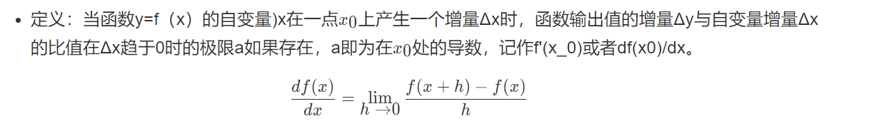
目的:使损失函数的值找到最小值
方式:梯度下降
函数的梯度(gradient)指出了函数的最陡增长方向。梯度的方向走,函数增长得就越快。那么按梯度的负方向走,函数值自然就降低得最快了。模型的训练目标即是寻找合适的 w 与 b 以最小化代价函数值。假设 w 与 b 都是一维实数,那么可以得到如下的 J 关于 w 与 b 的图:


可能根据简单的RMSE损失函数的是一个凸函数。但是一旦我们将函数扩展到神经网络,目标函数就就不再是凸函数了,图像也不会像上面那样是个碗状,而是凹凸不平的复杂地形形状。

注:在一篇论文中:Visualizing the Loss Landscape of Neural Nets,就专门做了将高位参数空间投影到二维或者三维的样子,这样投影之后的样子对神经网络的损失函数有个直观的认识,后面还会分析针对于这样的情况的优化问题。
2.4.2 神经网络的链式法则与反向传播算法
反向传播是训练神经网络最重要的算法,可以这么说,没有反向传播算法就没有深度学习的今天。但是反向传播算法设计一大堆数据公式概念。所以我们先复习回顾一下之前导数计算过程以及要介绍的新的复合函数多层求导计算过程。
- 导数、导数计算图
- 链式法则、逻辑回归的梯度下降优化、向量化编程
2.4.2.1 导数(复习)
2.4.2.2 导数计算理解(复习)
导数也可以理解成某一点处的斜率。斜率这个词更直观一些。
- 各点处的导数值一样

我们看到这里有一条直线,这条直线的斜率为4。我们来计算一个例子
例:取一点为a=2,那么y的值为8,我们稍微增加a的值为a=2.001,那么y的值为8.004,也就是当a增加了0.001,随后y增加了0.004,即4倍
那么我们的这个斜率可以理解为当一个点偏移一个不可估量的小的值,所增加的为4倍。

例:取一点为a=2,那么y的值为4,我们稍微增加a的值为a=2.001,那么y的值约等于4.004(4.004001),也就是当a增加了0.001,随后y增加了4倍
取一点为a=5,那么y的值为25,我们稍微增加a的值为a=5.001,那么y的值约等于25.01(25.010001),也就是当a增加了0.001,随后y增加了10倍
可以得出该函数的导数2为2a。
- 更多函数的导数结果

2.4.2.3 导数计算图


2.4.2.5 使用链式法则计算复合表达式
对于上面的例子,如果考虑更复杂的包含多个函数的复合函数,那么我们需要用到链式法则,指出将这些梯度表达式链接起来相乘。

那么整个计算图展示的就是计算过程,神经网络提到的前向传播就是从输入计算到输出(红色部分),反向传播从尾部开始,根据链式法则递归地向前计算梯度(显示为绿色),一直到网络的输入端。
- 反向传播总结
在反向传播的过程中,门单元门将最终获得整个网络的最终输出值在自己的输出值上的梯度。链式法则指出,门单元应该将回传的梯度乘以它对其的输入的局部梯度,从而得到整个网络的输出对该门单元的每个输入值的梯度。
2.4.2.6 案例:逻辑回归的链式法则推导过程
逻辑回归的梯度下降过程计算图,首先从前往后的计算图得出如下。


2.4.2.7 案例:逻辑回归前向与反向传播简单计算
假设简单的模型为y =sigmoid(w1x1+w2x2+b), 我们在这里给几个随机的输入的值和权重,带入来计算一遍,其中在点x1,x2 = (-1 -2),目标值为1,假设给一个初始化w1,w2,b=(2, -3, -3),由于中间有sigmoid的计算过程,所以我们用代码来呈现刚才的过程。
# 假设一些随机数据和权重,以及目标结果1
w = [2,-3,-3]
x = [-1, -2]
y = 1

# 前向传播
z = w[0]*x[0] + w[1]*x[1] + w[2]
a = 1.0 / (1 + np.exp(-z))
cost = -np.sum(y * np.log(a) + (1 - y) * np.log(1 - a))

# 对神经元反向传播
# 点积变量的梯度, 使用sigmoid函数求导
dz = a - y
# 回传计算x梯度
dx = [w[0] * dz, w[1] * dz]
# #回传计算w梯度
dw = [x[0] * dz, x[1] * dz, 1.0 * dz]
![]()
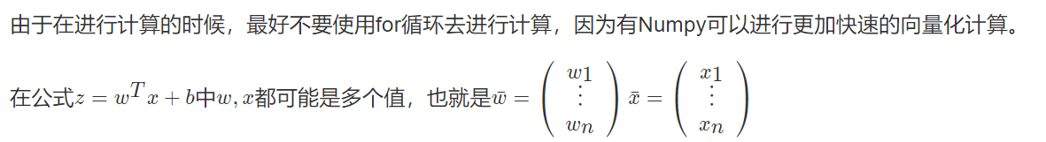
2.4.3 反向传播的向量化编程实现
每更新一次梯度时候,在训练期间我们会拥有m个样本,那么这样每个样本提供进去都可以做一个梯度下降计算。所以我们要去做在所有样本上的计算结果、梯度等操作


2.4.3.1 向量化优势
什么是向量化
import numpy as np
import time
a = np.random.rand(100000)
b = np.random.rand(100000)
- 第一种方法
# 第一种for 循环
c = 0
start = time.time()
for i in range(100000):
    c += a[i]*b[i]
end = time.time()

print("计算所用时间%s " % str(1000*(end-start)) + "ms")
- 第二种向量化方式使用np.dot
# 向量化运算
start = time.time()
c = np.dot(a, b)
end = time.time()
print("计算所用时间%s " % str(1000*(end-start)) + "ms")
Numpy能够充分的利用并行化,Numpy当中提供了很多函数使用
| 函数 | 作用 |
|---|---|
| np.ones or np.zeros | 全为1或者0的矩阵 |
| np.exp | 指数计算 |
| np.log | 对数计算 |
| np.abs | 绝对值计算 |
所以上述的m个样本的梯度更新过程,就是去除掉for循环。原本这样的计算
2.4.3.2 向量化反向传播实现伪代码


这相当于一次使用了M个样本的所有特征值与目标值,那我们知道如果想多次迭代,使得这M个样本重复若干次计算。
代码实现过程, 这里假设有10个样本,每个样本两个特征
# 随机初始化权重
# w1,w2
W = np.random.random([2, 1])
X = np.random.random([2, 10])
b = 0.0
Y = np.array([0, 1, 1, 0, 1, 1, 0, 1, 0, 0])

Z = np.dot(W.T, X) + b
A = 1.0 / (1 + np.exp(-Z))
cost = -1 / 10 * np.sum(Y * np.log(A) + (1 - Y) * np.log(1 - A))
# 形状:A:[1, 10] , Y:[1, 10]
dZ = A - Y
# [2, 10] * ([1, 10].T) = [2, 1]
dW = (1.0 / 10) * np.dot(X, dZ.T)
db = (1.0 / 10) * np.sum(dZ)
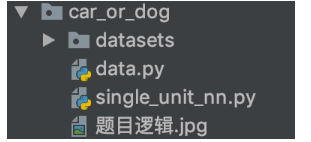
2.4.4 案例:实现单神经元神经网络
1、目的
读取猫狗的图片矩阵数据,自实现单神经元神经网络进行二分类
2、步骤
- 1、读取数据集
- 2、实现前向传播与反向传播过程
- 3、模型预测函数实现
3、代码实现
代码模块安排如下图
1、读取数据集以及主函数逻辑
import numpy as np
import h5py


def load_dataset():
    train_dataset = h5py.File('datasets/train_catvnoncat.h5', "r")
    train_set_x_orig = np.array(train_dataset["train_set_x"][:]) # your train set features
    train_set_y_orig = np.array(train_dataset["train_set_y"][:]) # your train set labels

    test_dataset = h5py.File('datasets/test_catvnoncat.h5', "r")
    test_set_x_orig = np.array(test_dataset["test_set_x"][:]) # your test set features
    test_set_y_orig = np.array(test_dataset["test_set_y"][:]) # your test set labels

    classes = np.array(test_dataset["list_classes"][:]) # the list of classes

    train_set_y_orig = train_set_y_orig.reshape((1, train_set_y_orig.shape[0]))
    test_set_y_orig = test_set_y_orig.reshape((1, test_set_y_orig.shape[0]))

    return train_set_x_orig, train_set_y_orig, test_set_x_orig, test_set_y_orig, classes
主体函数
导入相关包
import numpy as np
from data import load_dataset
主体逻辑
def main():

    # 1、读取样本数据
    train_x, train_y, test_x, test_y, classes = load_dataset()
    print("训练集的样本数: ", train_x.shape[0])
    print("测试集的样本数: ", test_x.shape[0])
    print("train_x形状: ", train_x.shape)
    print("train_y形状: ", train_y.shape)
    print("test_x形状: ", test_x.shape)
    print("test_x形状: ", test_y.shape)

    # 输入数据的形状修改以及归一化
    train_x = train_x.reshape(train_x.shape[0], -1).T
    test_x = test_x.reshape(test_x.shape[0], -1).T
    train_x = train_x / 255.
    test_x = test_x / 255.

    # 2、模型训练以及预测
    d = model(train_x, train_y, test_x, test_y, num_iterations=2000, learning_rate=0.005)
2、模型预测函数实现
模型函数
def model(X_train, Y_train, X_test, Y_test, num_iterations=2000, learning_rate=0.5):
    """
    """
    # 初始化参数
    w, b = initialize_with_zeros(X_train.shape[0])

    # 梯度下降
    # params:更新后的网络参数
    # grads:最后一次梯度
    # costs:每次更新的损失列表
    params, grads, costs = optimize(w, b, X_train, Y_train, num_iterations, learning_rate)

    # 获取训练的参数
    # 预测结果
    w = params['w']
    b = params['b']

    Y_prediction_train = predict(w, b, X_train)
    Y_prediction_test = predict(w, b, X_test)

    # 打印准确率
    print("训练集准确率: {} ".format(100 - np.mean(np.abs(Y_prediction_train - Y_train)) * 100))
    print("测试集准确率: {} ".format(100 - np.mean(np.abs(Y_prediction_test - Y_test)) * 100))

    d = {"costs": costs,
         "Y_prediction_test": Y_prediction_test,
         "Y_prediction_train": Y_prediction_train,
         "w": w,
         "b": b,
         "learning_rate": learning_rate,
         "num_iterations": num_iterations}

    return d
其中涉及两个函数一个是sigmoid另一个是初始化函数:
def basic_sigmoid(x):
    """
    计算sigmoid函数
    """

    s = 1 / (1 + np.exp(-x))

    return s


def initialize_with_zeros(shape):
    """
    创建一个形状为 (shape, 1) 的w参数和b=0.
    return:w, b
    """

    w = np.zeros((shape, 1))
    b = 0

    return w, b
3、前向传播与反向传播实现
def optimize(w, b, X, Y, num_iterations, learning_rate):
    """
    参数:
    w:权重,b:偏置,X特征,Y目标值,num_iterations总迭代次数,learning_rate学习率
    Returns:
    params:更新后的参数字典
    grads:梯度
    costs:损失结果
    """

    costs = []

    for i in range(num_iterations):

        # 梯度更新计算函数
        grads, cost = propagate(w, b, X, Y)

        # 取出两个部分参数的梯度
        dw = grads['dw']
        db = grads['db']

        # 按照梯度下降公式去计算
        w = w - learning_rate * dw
        b = b - learning_rate * db

        if i % 100 == 0:
            costs.append(cost)
        if i % 100 == 0:
            print("损失结果 %i: %f" % (i, cost))
            print(b)

    params = {"w": w,
              "b": b}

    grads = {"dw": dw,
             "db": db}

    return params, grads, costs

def propagate(w, b, X, Y):
    """
    参数:w,b,X,Y:网络参数和数据
    Return:
    损失cost、参数W的梯度dw、参数b的梯度db
    """
    m = X.shape[1]

    # 前向传播
    # w (n,1), x (n, m)
    A = basic_sigmoid(np.dot(w.T, X) + b)
    # 计算损失
    cost = -1 / m * np.sum(Y * np.log(A) + (1 - Y) * np.log(1 - A))

    # 反向传播
    dz = A - Y
    dw = 1 / m * np.dot(X, dz.T)
    db = 1 / m * np.sum(dz)

    grads = {"dw": dw,
             "db": db}

    return grads, cost
预测函数为:
def predict(w, b, X):
    '''
    利用训练好的参数预测

    return:预测结果
    '''

    m = X.shape[1]
    Y_prediction = np.zeros((1, m))
    w = w.reshape(X.shape[0], 1)

    # 计算结果
    A = basic_sigmoid(np.dot(w.T, X) + b)

    for i in range(A.shape[1]):

        if A[0, i] <= 0.5:
            Y_prediction[0, i] = 0
        else:
            Y_prediction[0, i] = 1

    assert (Y_prediction.shape == (1, m))

    return Y_prediction
运行结果显示:
训练集的样本数:  209
测试集的样本数:  50
train_x形状:  (209, 64, 64, 3)
train_y形状:  (1, 209)
test_x形状:  (50, 64, 64, 3)
test_x形状:  (1, 50)
损失结果 0: 0.693147
-0.000777511961722488
损失结果 100: 0.584508
-0.004382762341768198
损失结果 200: 0.466949
-0.006796745374030192
损失结果 300: 0.376007
-0.008966216045043067
损失结果 400: 0.331463
-0.010796335272035083
损失结果 500: 0.303273
-0.012282447313396519
损失结果 600: 0.279880
-0.013402386273819053
损失结果 700: 0.260042
-0.014245091216970799
损失结果 800: 0.242941
-0.014875420165524832
损失结果 900: 0.228004
-0.015341288386626626
损失结果 1000: 0.214820
-0.015678788375442378
损失结果 1100: 0.203078
-0.015915536343924556
损失结果 1200: 0.192544
-0.01607292624287493
损失结果 1300: 0.183033
-0.016167692508505707
损失结果 1400: 0.174399
-0.016213022073676534
损失结果 1500: 0.166521
-0.016219364232163875
损失结果 1600: 0.159305
-0.01619503271238927
损失结果 1700: 0.152667
-0.016146661324349904
损失结果 1800: 0.146542
-0.01607955397736277
损失结果 1900: 0.140872
-0.015997956805040348
训练集准确率: 99.04306220095694
测试集准确率: 70.0
2.4.5 总结
- 导数、导数计算图
- 链式法则、逻辑回归的梯度下降优化计算过程
data.py
import numpy as np
import h5py


def load_dataset():
    train_dataset = h5py.File('datasets/train_catvnoncat.h5', "r")
    train_set_x_orig = np.array(train_dataset["train_set_x"][:]) # your train set features
    train_set_y_orig = np.array(train_dataset["train_set_y"][:]) # your train set labels

    test_dataset = h5py.File('datasets/test_catvnoncat.h5', "r")
    test_set_x_orig = np.array(test_dataset["test_set_x"][:]) # your test set features
    test_set_y_orig = np.array(test_dataset["test_set_y"][:]) # your test set labels

    classes = np.array(test_dataset["list_classes"][:]) # the list of classes

    train_set_y_orig = train_set_y_orig.reshape((1, train_set_y_orig.shape[0]))
    test_set_y_orig = test_set_y_orig.reshape((1, test_set_y_orig.shape[0]))

    return train_set_x_orig, train_set_y_orig, test_set_x_orig, test_set_y_orig, classes
single_unit_nn.py
"""神经网络的模型读取训练过程
"""
import numpy as np
from data import load_dataset


def basic_sigmoid(x):
    """
    计算sigmoid函数
    """

    s = 1 / (1 + np.exp(-x))

    return s


def initialize_with_zeros(shape):
    """创建一个形状为(shape, 1)的权重参数
    :param shape: 特征值个数
    :return: w,b
    """

    w = np.zeros((shape, 1))
    b = 0

    return w, b


def propagate(w, b, X, Y):
    """单个神经元NN的前向传播和反向传播过程实现
    :param w: 权重 (shape, 1)
    :param b: 偏置
    :param X: 特征值
    :param Y: 目标值
    :return:grads, cost
    """
    m = X.shape[1]

    # 前向传播
    # w (64 * 64 * 3, 1), X (64 * 64 * 3, 209)
    A = basic_sigmoid(np.dot(w.T, X) + b)

    cost = -1 / m * np.sum(Y * np.log(A) + (1 - Y) * np.log(1 - A))

    # 反向传播
    dz = A - Y
    dw = 1 / m * np.dot(X, dz.T)
    db = 1 / m * np.sum(dz)

    grads = {
        "dw": dw,
        "db": db
    }

    return grads, cost


def optimize(w, b, train_x, train_y, num_iterations, learning_rate):
    """
    :param w: 训练的初始权重参数
    :param b: 训练初始偏置参数
    :param train_x: 训练集特征值
    :param train_y: 训练集目标值
    :param num_iterations: 迭代次数
    :param learning_rate: 学习率
    :return: params, grads, costs
    """
    costs = []

    # 训练迭代计算梯度,进行梯度下降公式更新
    for i in range(num_iterations):

        # 1、计算每次更新的梯度
        grads, cost = propagate(w, b, train_x, train_y)

        # 2、按照梯度更新公式进行更新
        # w = w - alpha* (dw)
        w = w - learning_rate * grads['dw']
        b = b - learning_rate * grads['db']

        # 打印结果
        if i % 100 == 0:
            costs.append(cost)
            print("损失结果第 %i 次, 值为: %f" % (i, cost))

    # 参数进行返回
    params = {
        "w": w,
        "b": b
    }

    grads = {
        "dw": grads['dw'],
        "db": grads['db']
    }

    return params, grads, costs


def predict(w, b, X):
    '''
    利用训练好的参数预测

    return:预测结果
    '''

    m = X.shape[1]
    Y_prediction = np.zeros((1, m))
    w = w.reshape(X.shape[0], 1)

    # 计算结果
    A = basic_sigmoid(np.dot(w.T, X) + b)

    for i in range(A.shape[1]):

        if A[0, i] <= 0.5:
            Y_prediction[0, i] = 0
        else:
            Y_prediction[0, i] = 1

    assert (Y_prediction.shape == (1, m))

    return Y_prediction


def model(train_x, train_y, test_x, test_y, num_iterations=2000, learning_rate=0.005):
    """
    :param train_x: 训练数据集特征值
    :param train_y: 训练数据集目标值
    :param test_x: 测试数据集特征值
    :param test_y: 测试数据集目标值
    :param num_iterations: 迭代次数
    :param learning_rate: 学习率
    :return:
    """
    # 1、初始化模型的参数
    w, b = initialize_with_zeros(train_x.shape[0])

    # 2、梯度下降的优化过程实现
    params, grads, costs = optimize(w, b, train_x, train_y, num_iterations, learning_rate)

    # 3、利用已训练好的模型参数进行预测,并计算出准确率
    Y_prediction_train = predict(params["w"], params["b"], train_x)
    Y_prediction_test = predict(params["w"], params["b"], test_x)

    # 计算准确率
    # 打印准确率
    print("训练集准确率: {} ".format(100 - np.mean(np.abs(Y_prediction_train - train_y)) * 100))
    print("测试集准确率: {} ".format(100 - np.mean(np.abs(Y_prediction_test - test_y)) * 100))

    d = {"costs": costs,
         "Y_prediction_test": Y_prediction_test,
         "Y_prediction_train": Y_prediction_train,
         "w": w,
         "b": b,
         "learning_rate": learning_rate,
         "num_iterations": num_iterations}

    return d


def main():

    # 1、读取样本数据
    train_x, train_y, test_x, test_y, classes = load_dataset()
    print("训练集的样本数: ", train_x.shape[0])
    print("测试集的样本数: ", test_x.shape[0])
    print("train_x形状: ", train_x.shape)
    print("train_y形状: ", train_y.shape)
    print("test_x形状: ", test_x.shape)
    print("test_x形状: ", test_y.shape)

    # 输入数据的形状修改以及归一化
    train_x = train_x.reshape(train_x.shape[0], -1).T
    test_x = test_x.reshape(test_x.shape[0], -1).T
    train_x = train_x / 255.
    test_x = test_x / 255.

    # 2、模型的训练以及预测过程
    d = model(train_x, train_y, test_x, test_y, num_iterations=2000, learning_rate=0.005)

    return None


if __name__ == '__main__':
    main()