logistic回归和softmax回归

logistic回归

在 logistic 回归中，我们的训练集由 $\textstyle m$ 个已标记的样本构成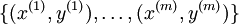： $\{ (x^{(1)}, y^{(1)}), \ldots, (x^{(m)}, y^{(m)}) \}$ 。由于 logistic 回归是针对二分类问题的，因此类标记 $y^{(i)} \in \{0,1\}$ 。

假设函数(hypothesis function): 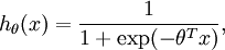$\begin{align}h_\theta(x) = \frac{1}{1+\exp(-\theta^Tx)},\end{align}$

代价函数(损失函数): $\begin{align}J(\theta) = -\frac{1}{m} \left[ \sum_{i=1}^m y^{(i)} \log h_\theta(x^{(i)}) + (1-y^{(i)}) \log (1-h_\theta(x^{(i)})) \right]\end{align}$

我们的目标是训练模型参数 $\textstyle \theta$ ，使其能够最小化代价函数。

假设函数就相当于我们在线性回归中要拟合的直线函数。

softmax回归

在 softmax回归中，我们的训练集由 $\textstyle m$ 个已标记的样本构成： $\{ (x^{(1)}, y^{(1)}), \ldots, (x^{(m)}, y^{(m)}) \}$ 。由于softmax回归是针对多分类问题（相对于 logistic 回归针对二分类问题），因此类标记 $\textstyle y$ 可以取 $\textstyle k$ 个不同的值（而不是 2 个）。我们有 $y^{(i)} \in \{1, 2, \ldots, k\}$ 。

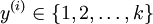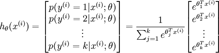
对于给定的测试输入 $\textstyle x$ ，我们想用假设函数针对每一个类别j估算出概率值 $\textstyle p(y=j | x)$ 。也就是说，我们想估计 $\textstyle x$ 的每一种分类结果出现的概率。因此，我们的假设函数将要输出一个 $\textstyle k$ 维的向量（向量元素的和为1）来表示这 $\textstyle k$ 个估计的概率值。具体地说，我们的假设函数 $\textstyle h_{\theta}(x)$ 形式如下：

假设函数： $\begin{align}h_\theta(x^{(i)}) =\begin{bmatrix}p(y^{(i)} = 1 | x^{(i)}; \theta) \\p(y^{(i)} = 2 | x^{(i)}; \theta) \\\vdots \\p(y^{(i)} = k | x^{(i)}; \theta)\end{bmatrix}=\frac{1}{ \sum_{j=1}^{k}{e^{ \theta_j^T x^{(i)} }} }\begin{bmatrix}e^{ \theta_1^T x^{(i)} } \\e^{ \theta_2^T x^{(i)} } \\\vdots \\e^{ \theta_k^T x^{(i)} } \\\end{bmatrix}\end{align}$

其中 $\theta_1, \theta_2, \ldots, \theta_k \in \Re^{n+1}$ 是模型的参数。请注意 $\frac{1}{ \sum_{j=1}^{k}{e^{ \theta_j^T x^{(i)} }} }$ 这一项对概率分布进行归一化，使得所有概率之和为 1 。

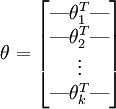
为了方便起见，我们同样使用符号 $\textstyle \theta$ 来表示全部的模型参数。在实现Softmax回归时，将 $\textstyle \theta$ 用一个 $\textstyle k \times(n+1)$ 的矩阵来表示会很方便，该矩阵是将 $\theta_1, \theta_2, \ldots, \theta_k$ 按行罗列起来得到的，如下所示：

$\theta = \begin{bmatrix}\mbox{---} \theta_1^T \mbox{---} \\\mbox{---} \theta_2^T \mbox{---} \\\vdots \\\mbox{---} \theta_k^T \mbox{---} \\\end{bmatrix}$

也就是说 $\textstyle h_{\theta}(x)$ 表示的是x属于不同类别的概率组成的向量。

代价函数： $\begin{align}J(\theta) = - \frac{1}{m} \left[ \sum_{i=1}^{m} \sum_{j=1}^{k} 1\left\{y^{(i)} = j\right\} \log \frac{e^{\theta_j^T x^{(i)}}}{\sum_{l=1}^k e^{ \theta_l^T x^{(i)} }}\right]\end{align}$

$\textstyle 1\{\cdot\}$ 是示性函数，其取值规则为

 值为真的表达式

值得注意的是，logistic回归代价函数是softmax代价函数的特殊情况。因此，logistic回归代价函数可以改为：

$\begin{align}J(\theta) &= -\frac{1}{m} \left[ \sum_{i=1}^m (1-y^{(i)}) \log (1-h_\theta(x^{(i)})) + y^{(i)} \log h_\theta(x^{(i)}) \right] \\&= - \frac{1}{m} \left[ \sum_{i=1}^{m} \sum_{j=0}^{1} 1\left\{y^{(i)} = j\right\} \log p(y^{(i)} = j | x^{(i)} ; \theta) \right]\end{align}$

一点个人理解：

为什么二分类中参数只有一个 $\textstyle \theta$ ，而k分类中参数却有k个。

其实二分类中的 $\textstyle \theta$ 是y=1情况下的参数，而y=0情况下其实未给出参数，因为y=0的假设函数值可以通过1-(y=1的假设函数值)得到。同理，k分类中参数其实只需要k-1个参数就可以了，多余的一个参数是冗余的。
具体冗余参数有什么负面影响，参考Softmax回归 http://ufldl.stanford.edu/wiki/index.php/Softmax%E5%9B%9E%E5%BD%92

知乎：https://www.zhihu.com/question/23765351

logistic回归和softmax回归

猜你喜欢