主要内容
1.BP神经网络概述
BP(Back Propagation)神经网络是1986年由Rumelhart和McCelland为首的科研小组提出,参见他们发表在Nature上的论文 Learning representations by back-propagating errors 。
BP神经网络是一种按误差逆传播算法训练的多层前馈网络,是目前应用最广泛的神经网络模型之一。BP网络能学习和存贮大量的 输入-输出模式映射关系,而无需事前揭示描述这种映射关系的数学方程。它的学习规则是使用最速下降法,通过反向传播来不断 调整网络的权值和阈值,使网络的误差平方和最小。
引用一位博主的话:在我看来BP神经网络就是一个”万能的模型+误差修正函数“,每次根据训练得到的结果与预想结果进行误差分析,进而修改权值和阈值,一步一步得到能输出和预想结果一致的模型。举一个例子:比如某厂商生产一种产品,投放到市场之后得到了消费者的反馈,根据消费者的反馈,厂商对产品进一步升级,优化,从而生产出让消费者更满意的产品。这就是BP神经网络的核心。
2.BP神经网络模型
BP神经网络是一种多层的前馈神经网络,其主要的特点是:信号是前向传播的,而误差是反向传播的。具体来说,对于如下的只含一个隐层的神经网络模型:
BP神经网络的过程主要分为两个阶段
第一阶段是信号的前向传播,从输入层经过隐含层,最后到达输出层;
第二阶段是误差的反向传播,从输出层到隐含层,最后到输入层,依次调节隐含层到输出层的权重和偏置,输入层到隐含层的权重和偏置。
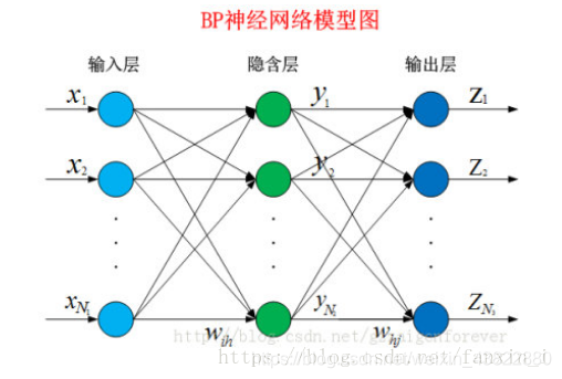
BP网络输入和输出的关系
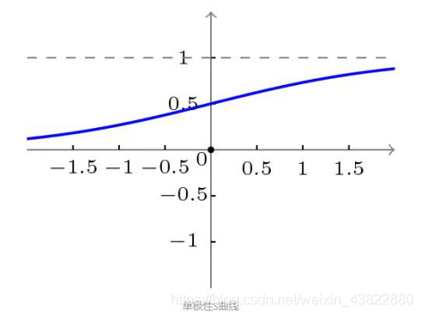
BP网络采用的传递函数是非线性变换函数——Sigmoid函数(又称S函数)。其特点是函数本身及其导数都是连续的,因而在处理上十分方便。为什么要选择这个函数,等下在介绍BP网络的学习算法的时候会进行进一步的介绍。S函数有单极性S型函数和双极性S型函数两种,单极性S型函数定义如下:f(x)=1/1+e−x
其函数曲线如图所示:
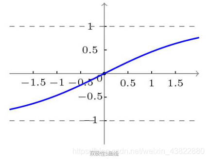
双极性S型函数:f(x)=1−e−x/1+e−x
使用S型激活函数时,输入:

输出:

输出的导数:
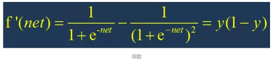
根据S激活函数的图形:
net在 -5~0 的时候导数的值为正,且导数的值逐渐增大,说明此时f(x)在逐渐变大 且 变大的速度越来越快
net在 0~5 的时候导数的值为正,且导数的值逐渐减小,说明此时f(x)在逐渐变大 但是 变大的速度越来越慢
对神经网络进行训练,我们应该尽量将net的值尽量控制在收敛比较快的范围内。
关于模型的详细公式推导,推荐这一篇:BP模型公式推导
3.BP神经网络策略
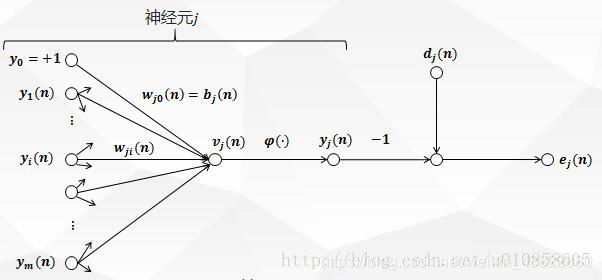
上图描绘了神经元jj被它左边的一层神经元产生的一组函数信号所馈给。mm是作用于神经元jj的所有输入不包括偏置的个数。突触权值wj0(n)wj0(n)等于神经元jj的偏置bjbj。
1.前向传播过程推导
图一中,在神经元jj的激活函数输入处产生的诱导局部域vj(n)vj(n)(即神经元jj 的输入)是:
ϕjϕj是激活函数,则出现在神经元jj输出处的函数信号(即神经元jj的输出)yj(n)yj(n)是:
2.误差反向传播过程推导
在图一中,yj(n)yj(n)与dj(n)dj(n)分别是神经元jj的实际输出和期望输出,则神经元jj的输出所产生的误差信号定义为:

其中,dj(n)dj(n)是期望响应向量d(n)d(n)的第jj个元素。
为了使函数连续可导,这里最小化均方根差,定义神经元jj的瞬时误差能量为:

将所有输出层神经元的误差能量相加,得到整个网络的全部瞬时误差能量:

其中,集合C 包括输出层的所有神经元。
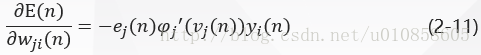
BP 算法通过反复修正权值使式(2-5)EnEn最小化,采用梯度下降法对突触权值wji(n)wji(n)应用一个修正值Δwji(n)∆wji(n)它正比于偏导数δδE(n)/E(n)/δδwji(n)wji(n)。根据微分链式规则,把这个梯度表示为:

偏导数δδE(n)/E(n)/δδwji(n)wji(n)代表一个敏感因子,决定突触权值wjiwji在权值空间的搜索方向。
在式(2-5)两边对ej(n)ej(n)取微分,得到:

在式(2-3)两边对yj(n)yj(n)取微分,得到:

在式(2-2)两边对vj(n)vj(n)取微分,得到:

最后在式(2-1)两边对wji(n)wji(n)取微分,得到:

将式(2-7)——(2-10)带入式(2-6)得:
应用于wji(n)wji(n)的修正Δwji(n)∆wji(n)定义为:

其中,ηη是误差反向传播的学习率, 负号表示在权空间中梯度下降。
将式(2-11)带入式(2-12)得:

其中,δj(n)δj(n)是根据delta法则定义的局部梯度:

局部梯度指明了突触权值所需要的变化。
现在来考虑神经元jj所处的层。
1) 神经元jj是输出层节点
当神经元jj位于输出层时,给它提供了一个期望响应。根据式(2-3)误差信号ej(n)=dj(n)−yj(n)ej(n)=dj(n)−yj(n)确定,通过式(2-14)得到神经元jj的局部梯度δj(n)δj(n)为:

2) 神经元jj是隐层节点
当神经元jj位于隐层时,没有对该输入神经元的指定期望响应。隐层的误差信号要根据所有与隐层神经元直接相连的神经元的误差信号向后递归决定。
考虑神经元jj为隐层节点,隐层神经元的局部梯度δj(n)δj(n)根据式(2-14)重新定义为:
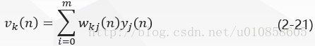
来看图二:它表示输出层神经元kk连接到隐层神经元jj的信号流图。

在这里下标jj表示隐层神经元,下标kk表示输出层神经元。
图二中,网络的全部瞬时误差能量为:

在式(2-17)两边对函数信号yj(n)yj(n)求偏导,得到:

在图二中:

因此,

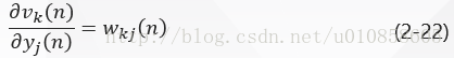
图二中,对于输出层神经元kk ,其诱导局部域是:
求式(2-21)对yj(n)yj(n)的微分得到:
将式(2-20)和(2-22)带入到式(2-18)得到:
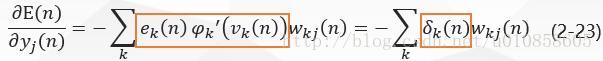
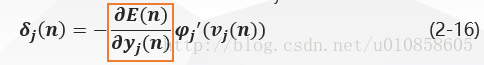
将式(2-23)带入式(2-16)得隐层神经元jj的局部梯度δj(n)δj(n)为:
反向传播过程推导总结
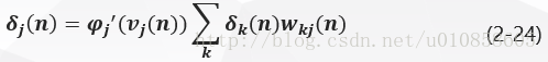
因此,结合式(2-13)、(2-15)和(2-24),由神经元ii连接到神经元jj的突触权值的修正值Δwji(n)∆wji(n)按照delta法则定义如下:

其中:
神经元jj是输出层节点时,局部梯度δj(n)δj(n)等于倒数ϕ′j(vj(n))ϕj′(vj(n))和误差信号ej(n)=dj(n)−yj(n)ej(n)=dj(n)−yj(n)的乘积,见式(2-15);
神经元jj是隐层节点时,局部梯度δj(n)δj(n)等于倒数ϕ′j(vj(n))ϕj′(vj(n))和下一层(隐层或输出层)的δkδk与权值加权和的乘积,见式(2-24)
此处参考博客
4.BP神经网络算法

5.BP神经网络MATLAB实现
神经网络运用到的函数
newff函数:
该函数用于创建一个前馈BP神经网络
net=newff(P,T,S,TF,BTF,BLF,PF,IPF,OPF,DDF)

sign函数:
该函数为符号函数 (Signum function)。
当x<0时,sign(x)=-1;
当x=0时,sign(x)=0;
当x>0时,sign(x)=1。
purelin函数是线性函数,y=a*x+b;
tansig函数是反正切函数y=1/(arctan(x)+1);
logsig函数是y=1/(1+e^(-x));
errsurf函数:单输入神经元的误差曲面。
plotes函数绘制单输入神经元的误差曲面。
epochs函数:定义神经网络net的循环次数
5.1构建BP神经网络
% BP网络
% BP神经网络的构建
net=newff([-1 2;0 5],[3,1],{'tansig','purelin'},'traingd')
net.IW{1}
net.b{1}

p=[1;2];
a=sim(net,p)
net=init(net);
net.IW{1}
net.b{1}
a=sim(net,p)
%net.IW{1}*p+net.b{1}
p2=net.IW{1}*p+net.b{1}
a2=sign(p2)
a3=tansig(a2)
a4=purelin(a3)
net.b{2}
net.b{1}

net.IW{1}
net.IW{2}
0.7616+net.b{2}
a-net.b{2}
(a-net.b{2})/ 0.7616
help purelin

p1=[0;0];
a5=sim(net,p1)
net.b{2}
运行结果:
>> BP
net =
   Neural Network
              name: 'Custom Neural Network'
          userdata: (your custom info)

    dimensions:

         numInputs: 1
         numLayers: 2
        numOutputs: 1
    numInputDelays: 0
    numLayerDelays: 0
 numFeedbackDelays: 0
 numWeightElements: 13
        sampleTime: 1

    connections:

       biasConnect: [1; 1]
      inputConnect: [1; 0]
      layerConnect: [0 0; 1 0]
     outputConnect: [0 1]

    subobjects:

             input: Equivalent to inputs{1}
            output: Equivalent to outputs{2}

            inputs: {1x1 cell array of 1 input}
            layers: {2x1 cell array of 2 layers}
           outputs: {1x2 cell array of 1 output}
            biases: {2x1 cell array of 2 biases}
      inputWeights: {2x1 cell array of 1 weight}
      layerWeights: {2x2 cell array of 1 weight}

    functions:

          adaptFcn: 'adaptwb'
        adaptParam: (none)
          derivFcn: 'defaultderiv'
         divideFcn: (none)
       divideParam: (none)
        divideMode: 'sample'
           initFcn: 'initlay'
        performFcn: 'mse'
      performParam: .regularization, .normalization
          plotFcns: {'plotperform', plottrainstate,
                    plotregression}
        plotParams: {1x3 cell array of 3 params}
          trainFcn: 'traingd'
        trainParam: .showWindow, .showCommandLine, .show, .epochs,
                    .time, .goal, .min_grad, .max_fail, .lr

    weight and bias values:

                IW: {2x1 cell} containing 1 input weight matrix
                LW: {2x2 cell} containing 1 layer weight matrix
                 b: {2x1 cell} containing 2 bias vectors

    methods:

             adapt: Learn while in continuous use
         configure: Configure inputs & outputs
            gensim: Generate Simulink model
              init: Initialize weights & biases
           perform: Calculate performance
               sim: Evaluate network outputs given inputs
             train: Train network with examples
              view: View diagram
       unconfigure: Unconfigure inputs & outputs


ans =

    0.9793    0.7717
    1.5369    0.3008
   -1.0989   -0.7114


ans =

   -4.8438
   -1.5204
   -0.0970


a =

    0.5105


ans =

   -1.6151   -0.0414
    1.3628    0.5217
    1.2726   -0.5981


ans =

    3.3359
   -1.9858
    3.2839


a =

    1.6873


p2 =

    1.6380
    0.4205
    3.3602


a2 =

     1
     1
     1


a3 =

    0.7616
    0.7616
    0.7616


a4 =

    0.7616
    0.7616
    0.7616


ans =

    0.9190


ans =

    3.3359
   -1.9858
    3.2839


ans =

   -1.6151   -0.0414
    1.3628    0.5217
    1.2726   -0.5981


ans =

     []


ans =

    1.6806


ans =

    0.7683


ans =

    1.0088

a5 =

    0.5450


ans =

    0.9190

>>
BP神经网络的构建
% BP网络
% BP神经网络的构建
net=newff([-1 2;0 5],[3,1],{'tansig','purelin'},'traingd')
net.IW{1}
net.b{1}
%p=[1;];
p=[1;2];
a=sim(net,p)
net=init(net);
net.IW{1}
net.b{1}
a=sim(net,p)
net.IW{1}*p+net.b{1}
p2=net.IW{1}*p+net.b{1}
a2=sign(p2)
a3=tansig(a2)
a4=purelin(a3)
net.b{2}
net.b{1}

P=[1.2;3;0.5;1.6]
W=[0.3 0.6 0.1 0.8]
net1=newp([0 2;0 2;0 2;0 2],1,'purelin');
net2=newp([0 2;0 2;0 2;0 2],1,'logsig');
net3=newp([0 2;0 2;0 2;0 2],1,'tansig');
net4=newp([0 2;0 2;0 2;0 2],1,'hardlim');

net1.IW{1}
net2.IW{1}
net3.IW{1}
net4.IW{1}
net1.b{1}
net2.b{1}
net3.b{1}
net4.b{1}


net1.IW{1}=W;
net2.IW{1}=W;
net3.IW{1}=W;
net4.IW{1}=W;

a1=sim(net1,P)
a2=sim(net2,P)
a3=sim(net3,P)
a4=sim(net4,P)

init(net1);
net1.b{1}

help tansig
运行结果:
>> BP
net =
   Neural Network

              name: 'Custom Neural Network'
          userdata: (your custom info)

    dimensions:

         numInputs: 1
         numLayers: 2
        numOutputs: 1
    numInputDelays: 0
    numLayerDelays: 0
 numFeedbackDelays: 0
 numWeightElements: 13
        sampleTime: 1

    connections:

       biasConnect: [1; 1]
      inputConnect: [1; 0]
      layerConnect: [0 0; 1 0]
     outputConnect: [0 1]

    subobjects:

             input: Equivalent to inputs{1}
            output: Equivalent to outputs{2}

            inputs: {1x1 cell array of 1 input}
            layers: {2x1 cell array of 2 layers}
           outputs: {1x2 cell array of 1 output}
            biases: {2x1 cell array of 2 biases}
      inputWeights: {2x1 cell array of 1 weight}
      layerWeights: {2x2 cell array of 1 weight}

    functions:

          adaptFcn: 'adaptwb'
        adaptParam: (none)
          derivFcn: 'defaultderiv'
         divideFcn: (none)
       divideParam: (none)
        divideMode: 'sample'
           initFcn: 'initlay'
        performFcn: 'mse'
      performParam: .regularization, .normalization
          plotFcns: {'plotperform', plottrainstate,
                    plotregression}
        plotParams: {1x3 cell array of 3 params}
          trainFcn: 'traingd'
        trainParam: .showWindow, .showCommandLine, .show, .epochs,
                    .time, .goal, .min_grad, .max_fail, .lr

    weight and bias values:

                IW: {2x1 cell} containing 1 input weight matrix
                LW: {2x2 cell} containing 1 layer weight matrix
                 b: {2x1 cell} containing 2 bias vectors

    methods:

             adapt: Learn while in continuous use
         configure: Configure inputs & outputs
            gensim: Generate Simulink model
              init: Initialize weights & biases
           perform: Calculate performance
               sim: Evaluate network outputs given inputs
             train: Train network with examples
              view: View diagram
       unconfigure: Unconfigure inputs & outputs


ans =

   -0.3285    0.9497
   -0.5719   -0.9072
    1.6154   -0.0374


ans =

    0.2148
    2.5540
    1.7106


a =

    0.8726


ans =

   -0.8941   -0.8081
    0.6896   -0.8773
    1.6165   -0.0102


ans =

    4.8922
    1.8484
    1.6422


a =

    0.3126


ans =

    2.3819
    0.7834
    3.2382


p2 =

    2.3819
    0.7834
    3.2382


a2 =

     1
     1
     1


a3 =

    0.7616
    0.7616
    0.7616


a4 =

    0.7616
    0.7616
    0.7616


ans =

   -0.5524


ans =

    4.8922
    1.8484
    1.6422


P =

    1.2000
    3.0000
    0.5000
    1.6000


W =

    0.3000    0.6000    0.1000    0.8000


ans =

     0     0     0     0


ans =

     0     0     0     0


ans =

     0     0     0     0


ans =

     0     0     0     0


ans =

     0


ans =

     0


ans =

     0


ans =

     0


a1 =

    3.4900


a2 =

    0.9704


a3 =

    0.9981


a4 =

     1


ans =

     0

>>
5.2 BP神经网络的训练
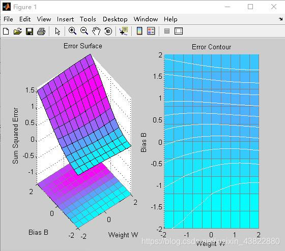
p=[-0.1 0.5]
t=[-0.3 0.4]
w_range=-2:0.4:2;
b_range=-2:0.4:2;
ES=errsurf(p,t,w_range,b_range,'logsig');%单输入神经元的误差曲面
plotes(w_range,b_range,ES)%绘制单输入神经元的误差曲面
pause(0.5);
hold off;
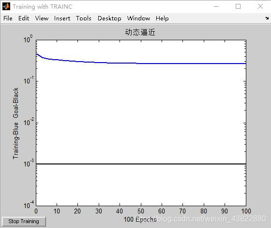
net=newp([-2,2],1,'logsig');
net.trainparam.epochs=100;
net.trainparam.goal=0.001;
figure(2);
[net,tr]=train(net,p,t);
title('动态逼近')
wight=net.iw{1}
bias=net.b
pause;
close;
运行结果:
>> BP

p =

   -0.1000    0.5000


t =

   -0.3000    0.4000


wight =

   15.1653


bias =

    [-8.8694]

% 训练
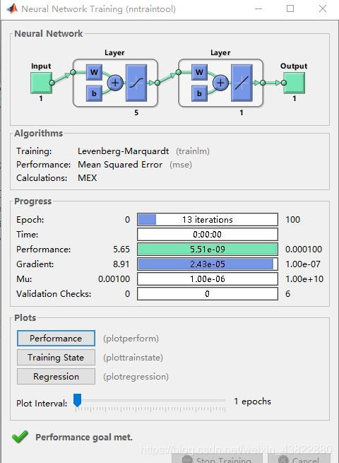
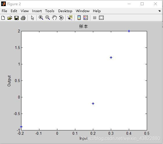
p=[-0.2 0.2 0.3 0.4]
t=[-0.9 -0.2 1.2 2.0]
h1=figure(1);
net=newff([-2,2],[5,1],{'tansig','purelin'},'trainlm');
net.trainparam.epochs=100;
net.trainparam.goal=0.0001;
net=train(net,p,t);
a1=sim(net,p)
pause;
h2=figure(2);
plot(p,t,'*');
title('样本')
title('样本');
xlabel('Input');
ylabel('Output');
pause;
hold on;
ptest1=[0.2 0.1]
ptest2=[0.2 0.1 0.9]
a1=sim(net,ptest1);
a2=sim(net,ptest2);
net.iw{1}
net.iw{2}
net.b{1}
net.b{2}
运行结果:
>> BP

p =

   -0.2000    0.2000    0.3000    0.4000


t =

   -0.9000   -0.2000    1.2000    2.0000


a1 =

   -0.9000   -0.1999    1.1999    2.0000


ptest1 =

    0.2000    0.1000


ptest2 =

    0.2000    0.1000    0.9000


ans =

    3.4994
    9.9514
    3.7383
    3.4868
    3.5000


ans =

     []


ans =

   -7.0014
   -2.6098
    3.3197
    3.4796
    7.0000


ans =

   -0.1984

>>
6.BP神经网络可能遇到的问题