一、机器学习概览
0 检查版本信息
import sys
assert sys.version_info >= (3, 5)
sys.version_info

import sklearn
assert sklearn.__version__ >= "0.20"
sklearn.__version__

1 获取数据并整理
1.1 下载数据
创建
datasets/lifesat目录
爬取oecd_bli_2015.csv&gdp_per_capita.csv数据到该目录下
import os
datapath = os.path.join("datasets", "lifesat", "") # 拼接

import urllib
DOWNLOAD_ROOT = "https://raw.githubusercontent.com/ageron/handson-ml2/master/"
os.makedirs(datapath, exist_ok=True)
for filename in ("oecd_bli_2015.csv", "gdp_per_capita.csv"):
    print("Downloading", filename)
    url = DOWNLOAD_ROOT + "datasets/lifesat/" + filename
    urllib.request.urlretrieve(url, datapath + filename)

!tree datasets
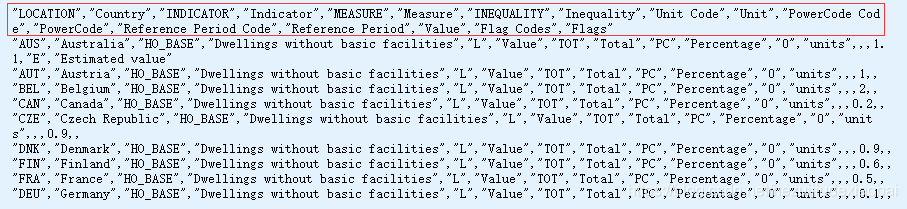
!head -10 datasets/lifesat//oecd_bli_2015.csv
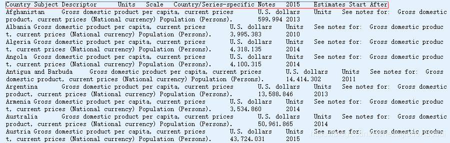
!head -10 datasets/lifesat//gdp_per_capita.csv
1.2 加载数据
pd.read_csv
thousands: str, default None
<>Thousands separator.
delimiter: str, defaultNone
<>Alternative argument name for sep.
encoding: str, default None
<>Encoding to use for UTF when reading/writing (ex. ‘utf-8’). List of Python standard encodings
na_values: scalar, str, list-like, or dict, default None
<>Additional strings to recognize as NA/NaN. If dict passed, specific
per-column NA values. By default the following values are interpreted as
NaN: ‘’, ‘#N/A’, ‘#N/A N/A’, ‘#NA’, ‘-1.#IND’, ‘-1.#QNAN’, ‘-NaN’, ‘-nan’,
‘1.#IND’, ‘1.#QNAN’, ‘N/A’, ‘NA’, ‘NULL’, ‘NaN’, ‘n/a’, ‘nan’,
‘null’.
import matplotlib.pyplot as plt
import numpy as np
import pandas as pd
import sklearn.linear_model
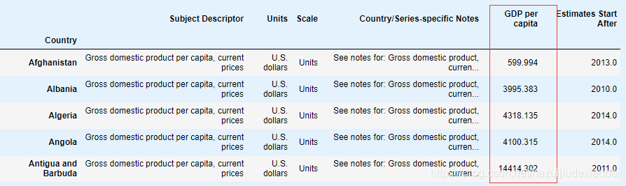
oecd_bli = pd.read_csv(datapath + "oecd_bli_2015.csv", thousands=',')
gdp_per_capita = pd.read_csv(datapath + "gdp_per_capita.csv", thousands=',',delimiter='\t',
encoding='latin1', na_values="n/a")
oecd_bli.info()
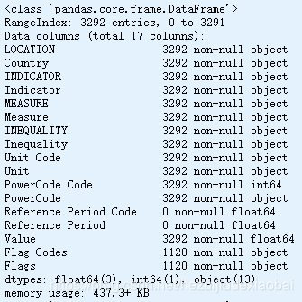
oecd_bli.shape

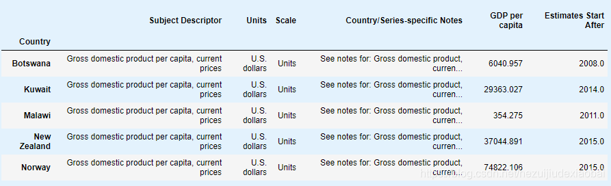
gdp_per_capita.info()
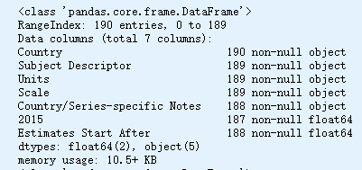
gdp_per_capita.shape

直接下载数据
import pandas as pd
oecd_bli_ = pd.read_csv("https://raw.githubusercontent.com/ageron/handson-ml/master/datasets/lifesat/oecd_bli_2015.csv", thousands=',')

oecd_bli_.shape

import pandas as pd
gdp_per_capita_ = pd.read_csv("https://raw.githubusercontent.com/ageron/handson-ml/master/datasets/lifesat/gdp_per_capita.csv",
                        thousands=',',delimiter='\t', encoding='latin1', na_values="n/a")

gdp_per_capita_.shape

1.3 预处理数据
将
OECD's(经合组织)生活满意度数据和IMF's(国际货币基金组织)的人均GDP数据合并在一起
pd.DataFrame.pivot
pd.DataFrame.rename
pd.DataFrame.set_index
pd.DataFrame.merge
pd.DataFrame.sort_values
def prepare_country_stats(oecd_bli, gdp_per_capita):
    oecd_bli = oecd_bli[oecd_bli["INEQUALITY"]=="TOT"] # 过滤
    oecd_bli = oecd_bli.pivot(index="Country", columns="Indicator", values="Value") # 透视
    gdp_per_capita.rename(columns={"2015": "GDP per capita"}, inplace=True) # 更改轴标签
    gdp_per_capita.set_index("Country", inplace=True) # 重置索引
    full_country_stats = pd.merge(left=oecd_bli, right=gdp_per_capita,
                                  left_index=True, right_index=True) # 合并
    full_country_stats.sort_values(by="GDP per capita", inplace=True) # 排序
    remove_indices = [0, 1, 6, 8, 33, 34, 35] # 移除某些国家
    keep_indices = list(set(range(36)) - set(remove_indices))
    return full_country_stats[["GDP per capita", 'Life satisfaction']].iloc[keep_indices] # 全部国家信息
np.c_
country_stats = prepare_country_stats(oecd_bli, gdp_per_capita)
X = np.c_[country_stats["GDP per capita"]]
y = np.c_[country_stats["Life satisfaction"]]
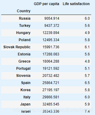
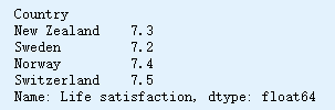
country_stats
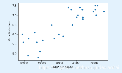
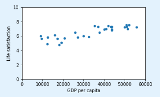
1.4 数据可视化
country_stats.plot(kind='scatter', x="GDP per capita", y='Life satisfaction')
plt.show()
1.5 线性回归模型
# 线性回归模型
model = sklearn.linear_model.LinearRegression()
# 训练
model.fit(X, y)
# 预测
X_new = [[22587]]
model.predict(X_new)
2 基于模型学习
保存图片
PROJECT_ROOT_DIR = "."
CHAPTER_ID = "fundamentals"
IMAGES_PATH = os.path.join(PROJECT_ROOT_DIR, "images", CHAPTER_ID) # 拼接
os.makedirs(IMAGES_PATH, exist_ok=True) # 创建目录

def save_fig(fig_id, tight_layout=True, fig_extension="png", resolution=300):
    path = os.path.join(IMAGES_PATH, fig_id + "." + fig_extension) # 拼接
    print("Saving figure", fig_id)
    if tight_layout:
        plt.tight_layout() # 最佳位置
    plt.savefig(path, format=fig_extension, dpi=resolution)

!ls images

2.1 读取并准备Life satisfaction数据
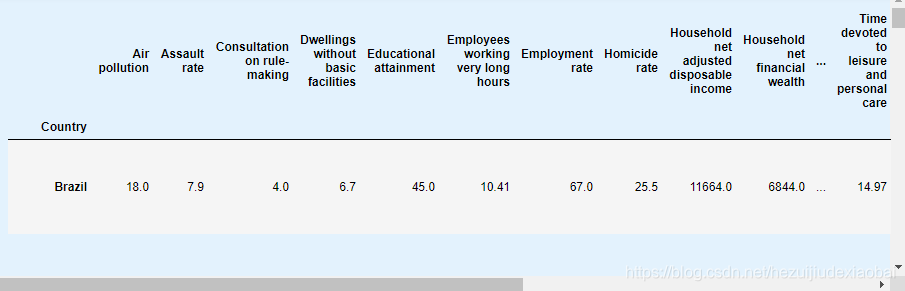
oecd_bli = pd.read_csv(datapath + "oecd_bli_2015.csv", thousands=',')
oecd_bli = oecd_bli[oecd_bli["INEQUALITY"]=="TOT"]
oecd_bli = oecd_bli.pivot(index="Country", columns="Indicator", values="Value")
oecd_bli.head()
2.2 读取并准备GDP per capita数据
gdp_per_capita = pd.read_csv(datapath+"gdp_per_capita.csv", thousands=',', delimiter='\t',
                             encoding='latin1', na_values="n/a")
gdp_per_capita.rename(columns={"2015": "GDP per capita"}, inplace=True)
gdp_per_capita.set_index("Country", inplace=True)
gdp_per_capita.head()
2.3 合并Life satisfaction & GDP per capita数据
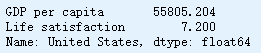
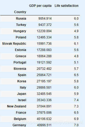
full_country_stats = pd.merge(left=oecd_bli, right=gdp_per_capita, left_index=True, right_index=True)
full_country_stats.sort_values(by="GDP per capita", inplace=True)
full_country_stats
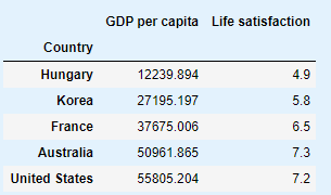
full_country_stats[["GDP per capita", 'Life satisfaction']].loc["United States"]
2.4 分割数据集
remove_indices = [0, 1, 6, 8, 33, 34, 35]
keep_indices = list(set(range(36)) - set(remove_indices))
sample_data = full_country_stats[["GDP per capita", 'Life satisfaction']].iloc[keep_indices]
missing_data = full_country_stats[["GDP per capita", 'Life satisfaction']].iloc[remove_indices]
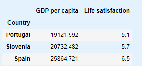
sample_data
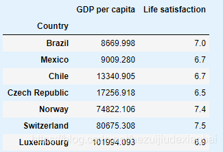
missing_data # 移除的国家数据
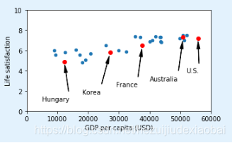
2.5 用一些国家画图
dict.items # 返回可遍历的(键, 值) 元组数组
plt.annotate # 用文本注释点
sample_data.plot(kind='scatter', x="GDP per capita", y='Life satisfaction', figsize=(5,3))
plt.axis([0, 60000, 0, 10])
sample_data.plot(kind='scatter', x="GDP per capita", y='Life satisfaction', figsize=(5,3))
plt.axis([0, 60000, 0, 10]) # 设置轴属性
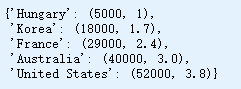
position_text = { # 文本&文本位置
"Hungary": (5000, 1),
"Korea": (18000, 1.7),
"France": (29000, 2.4),
"Australia": (40000, 3.0),
"United States": (52000, 3.8),
}
for country, pos_text in position_text.items(): # 字典 dict.items
pos_data_x, pos_data_y = sample_data.loc[country] # 数据
country = "U.S." if country == "United States" else country # United States -> U.S.
plt.annotate(country, xy=(pos_data_x, pos_data_y), xytext=pos_text,
arrowprops=dict(facecolor='black', width=0.5, shrink=0.1, headwidth=5)) # 用文本注释点
plt.plot(pos_data_x, pos_data_y, "ro")
plt.xlabel("GDP per capita (USD)")
save_fig('money_happy_scatterplot') # 保存
plt.show()
2.6 线性模型
sample_data.to_csv(os.path.join("datasets", "lifesat", "lifesat.csv"))

position_text
sample_data.loc[list(position_text.keys())]
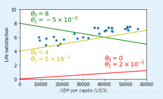
sample_data.plot(kind='scatter', x="GDP per capita", y='Life satisfaction', figsize=(5,3))
plt.xlabel("GDP per capita (USD)")
plt.axis([0, 60000, 0, 10])
X=np.linspace(0, 60000, 1000)

plt.plot(X, 2*X/100000, "r")
plt.text(40000, 2.7, r"$\theta_0 = 0$", fontsize=14, color="r")
plt.text(40000, 1.8, r"$\theta_1 = 2 \times 10^{-5}$", fontsize=14, color="r")

plt.plot(X, 8 - 5*X/100000, "g")
plt.text(5000, 9.1, r"$\theta_0 = 8$", fontsize=14, color="g")
plt.text(5000, 8.2, r"$\theta_1 = -5 \times 10^{-5}$", fontsize=14, color="g")

plt.plot(X, 4 + 5*X/100000, "y")
plt.text(5000, 3.5, r"$\theta_0 = 4$", fontsize=14, color="y")
plt.text(5000, 2.6, r"$\theta_1 = 5 \times 10^{-5}$", fontsize=14, color="y")

save_fig('tweaking_model_params_plot')
plt.show()
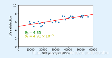
2.7 模型训练
from sklearn import linear_model
lin1 = linear_model.LinearRegression()
Xsample = np.c_[sample_data["GDP per capita"]]
ysample = np.c_[sample_data["Life satisfaction"]]
lin1.fit(Xsample, ysample)
t0, t1 = lin1.intercept_[0], lin1.coef_[0][0]
t0, t1

最佳拟合训练数据的线性模型
sample_data.plot(kind='scatter', x="GDP per capita", y='Life satisfaction', figsize=(5,3))

plt.xlabel("GDP per capita (USD)")
plt.axis([0, 60000, 0, 10])

X=np.linspace(0, 60000, 1000)
plt.plot(X, t0 + t1*X, "r")
plt.text(5000, 3.1, r"$\theta_0 = 4.85$", fontsize=14, color="g")
plt.text(5000, 2.2, r"$\theta_1 = 4.91 \times 10^{-5}$", fontsize=14, color="y")
save_fig('best_fit_model_plot')
plt.show()
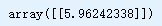
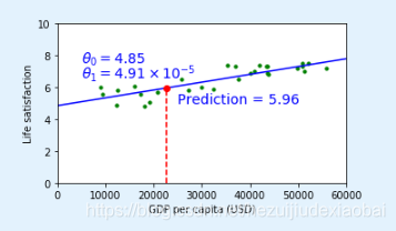
2.8 对Cyprus进行预测
塞浦路斯 地中海东部之一岛国,原属英,1960年独立,首都Nicosia
cyprus_predicted_life_satisfaction = lin1.predict([[cyprus_gdp_per_capita]])[0][0]
cyprus_predicted_life_satisfaction

sample_data.plot(kind='scatter', x="GDP per capita", y='Life satisfaction', figsize=(5,3), s=10, c='g')

plt.xlabel("GDP per capita (USD)")
X=np.linspace(0, 60000, 1000)
plt.plot(X, t0 + t1*X, "b")
plt.axis([0, 60000, 0, 10])
plt.text(5000, 7.5, r"$\theta_0 = 4.85$", fontsize=14, color="b")
plt.text(5000, 6.6, r"$\theta_1 = 4.91 \times 10^{-5}$", fontsize=14, color="b")

plt.plot([cyprus_gdp_per_capita, cyprus_gdp_per_capita], [0, cyprus_predicted_life_satisfaction], "r--") # 虚线
plt.text(25000, 5.0, r"Prediction = 5.96", fontsize=14, color="b")
plt.plot(cyprus_gdp_per_capita, cyprus_predicted_life_satisfaction, "ro")
save_fig('cyprus_prediction_plot')
plt.show()
分析
sample_data[7:10]
gdp_per_capita.loc["Cyprus"]["GDP per capita"]

SloveniaCyprus(GDP per capita)
sample_data[7:10]['Life satisfaction'].mean()

预测值很接近
2.9 K近邻回归
import sklearn.neighbors
model = sklearn.neighbors.KNeighborsRegressor(n_neighbors=3)

X = np.c_[country_stats["GDP per capita"]]
y = np.c_[country_stats["Life satisfaction"]]

# Train the model
model.fit(X, y)

# Make a prediction for Cyprus
X_new = np.array([[22587.0]])  # Cyprus' GDP per capita
print(model.predict(X_new)) # outputs [[ 5.76666667]]

3 机器学习的主要挑战
3.1 没有代表性的训练数据
backup = oecd_bli, gdp_per_capita # 备份
def prepare_country_stats(oecd_bli, gdp_per_capita):
oecd_bli = oecd_bli[oecd_bli["INEQUALITY"]=="TOT"] # 过滤
oecd_bli = oecd_bli.pivot(index="Country", columns="Indicator", values="Value") # 透视
gdp_per_capita.rename(columns={"2015": "GDP per capita"}, inplace=True) # 更改轴标签
gdp_per_capita.set_index("Country", inplace=True) # 重置索引
full_country_stats = pd.merge(left=oecd_bli, right=gdp_per_capita,
left_index=True, right_index=True) # 合并
full_country_stats.sort_values(by="GDP per capita", inplace=True) # 排序
remove_indices = [0, 1, 6, 8, 33, 34, 35] # 移除某些国家
keep_indices = list(set(range(36)) - set(remove_indices))
return full_country_stats[["GDP per capita", 'Life satisfaction']].iloc[keep_indices] # 全部国家信息
oecd_bli, gdp_per_capita = backup # 回滚
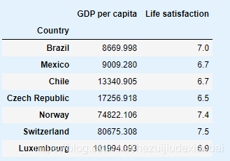
missing_data
position_text2 = {
    "Brazil": (1000, 9.0),
    "Mexico": (11000, 9.0),
    "Chile": (25000, 9.0),
    "Czech Republic": (35000, 9.0),
    "Norway": (60000, 3),
    "Switzerland": (72000, 3.0),
    "Luxembourg": (90000, 3.0),
}

sample_data.plot(kind='scatter', x="GDP per capita", y='Life satisfaction', figsize=(8,3))
plt.axis([0, 110000, 0, 10])

for country, pos_text in position_text2.items():
    pos_data_x, pos_data_y = missing_data.loc[country]
    plt.annotate(country, xy=(pos_data_x, pos_data_y), xytext=pos_text,
            arrowprops=dict(facecolor='black', width=0.5, shrink=0.1, headwidth=5))
    plt.plot(pos_data_x, pos_data_y, "rs")

X=np.linspace(0, 110000, 1000)
plt.plot(X, t0 + t1*X, "b:")

lin_reg_full = linear_model.LinearRegression()
Xfull = np.c_[full_country_stats["GDP per capita"]]
yfull = np.c_[full_country_stats["Life satisfaction"]]
lin_reg_full.fit(Xfull, yfull)

t0full, t1full = lin_reg_full.intercept_[0], lin_reg_full.coef_[0][0]
X = np.linspace(0, 110000, 1000)
plt.plot(X, t0full + t1full * X, "k")
plt.xlabel("GDP per capita (USD)")

save_fig('representative_training_data_scatterplot')
plt.show()
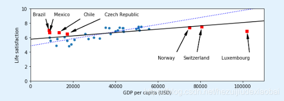
样本偏差
添加缺失国家后,发现一些贫穷国家看上去比富裕的国家还幸福
3.2 过拟合训练数据
full_country_stats.plot(kind='scatter', x="GDP per capita", y='Life satisfaction', figsize=(8,3))
plt.axis([0, 110000, 0, 10])

from sklearn import preprocessing
from sklearn import pipeline

poly = preprocessing.PolynomialFeatures(degree=60, include_bias=False) # 生成多项式特征
scaler = preprocessing.StandardScaler()
lin_reg2 = linear_model.LinearRegression()

pipeline_reg = pipeline.Pipeline([('poly', poly), ('scal', scaler), ('lin', lin_reg2)]) # 管道
pipeline_reg.fit(Xfull, yfull)
curve = pipeline_reg.predict(X[:, np.newaxis])
plt.plot(X, curve)
plt.xlabel("GDP per capita (USD)")
save_fig('overfitting_model_plot')
plt.show()
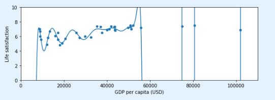
过度归纳
3.3 正则化
full_country_stats.loc[[c for c in full_country_stats.index if "W" in c.upper()]]["Life satisfaction"]
gdp_per_capita.loc[[c for c in gdp_per_capita.index if "W" in c.upper()]].head()
plt.figure(figsize=(8,3))

plt.xlabel("GDP per capita")
plt.ylabel('Life satisfaction')

plt.plot(list(sample_data["GDP per capita"]), list(sample_data["Life satisfaction"]), "bo")
plt.plot(list(missing_data["GDP per capita"]), list(missing_data["Life satisfaction"]), "rs")

X = np.linspace(0, 110000, 1000)
plt.plot(X, t0full + t1full * X, "r--", label="Linear model on all data")
plt.plot(X, t0 + t1*X, "g:", label="Linear model on partial data")

ridge = linear_model.Ridge(alpha=10**9.5) # 岭回归
Xsample = np.c_[sample_data["GDP per capita"]]
ysample = np.c_[sample_data["Life satisfaction"]]
ridge.fit(Xsample, ysample)
t0ridge, t1ridge = ridge.intercept_[0], ridge.coef_[0][0]
plt.plot(X, t0ridge + t1ridge * X, "b", label="Regularized linear model on partial data")

plt.legend(loc="lower right")
plt.axis([0, 110000, 0, 10])
plt.xlabel("GDP per capita (USD)")
save_fig('ridge_model_plot')
plt.show()
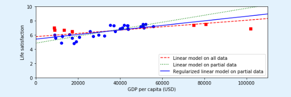
正则化降低了过度拟合的风险
