WGAN and WGAN-GP：Wasserstein GAN and Improved Training of Wasserstein GANs

Wasserstein GAN and Improved Training of Wasserstein GANs

Paper:
WGAN:https://arxiv.org/pdf/1701.07875.pdf
WGAN-GP:https://arxiv.org/pdf/1704.00028.pdf
参考：
https://lilianweng.github.io/lil-log/2017/08/20/from-GAN-to-WGAN.html
https://vincentherrmann.github.io/blog/wasserstein/
recommend:https://www.depthfirstlearning.com/2019/WassersteinGAN
（阅读笔记）

1.Intro

• 得到目标概率密度一般就利用极大似然估计的方法，而不同分布之间则一般用散度衡量。
• 模型生成得到的分布与原始真实的分布不太可能有交叉的地方。两个分布都仅仅只是各自有各自的，而不是联合的，得到的这种形式的目标分布是不理想的。It is then unlikely that…have a non-negligible intersection.
  • 所以很多文献都是通过给目标分布添加噪声来尽量覆盖所有的例子，但是会使图像受损。
  • 而GAN就是通过生成器让低维流形产生高维的分布，当下效果也不是很理想。
• 主要目标是衡量分布之间的距离。we direct our attention on the various ways to measure how close the model distribution and the real distribution are, or equivalently.
• 研究了EM距离。we provide a comprehensive theoretical analysis of how the Earth Mover (EM) distance behaves in comparison to popular probability distances and divergences used in the context of learning distributions.
• 定义了WGAN。we de fine a form of GAN called Wasserstein-GAN that minimizes a reasonable and efficient approximation of the EM distance, and we theoretically show that the corresponding optimization problem is sound.

2.Distances

• 各种 $distances(divergences)$： $\mathbf{TV}$； $\mathbf{KL}$； $\mathbf{JS}$等（可见论文 $f$-GAN），而 $Earth$- $Mover(EM)$如下：
  $\begin{aligned} W(\mathbb{P}_{r},\mathbb{P}_{g})&=\inf_{\gamma \in \Pi(\mathbb{P}_{r},\mathbb{P}_{g})} \mathbb{E}_{(x,y) \sim \gamma} \left[\|x-y \| \right]\\ &=\inf_{\gamma \in \Pi(\mathbb{P}_{r},\mathbb{P}_{g})} \int \int \left[\ \gamma(x,y)\|x-y \| \right]\mathrm{d}x\mathrm{d}y \tag{1} \end{aligned}$
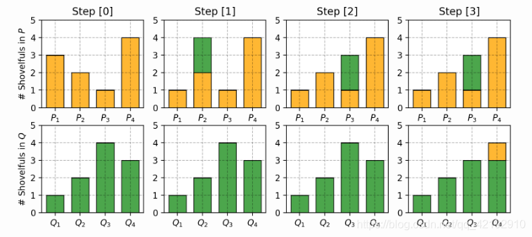
  $\mathbb{P}_{r},\mathbb{P}_{g}$的联合分布集为 $\Pi$； $\gamma$是其中一种联合分布；从 $\gamma$中抽样得到所有 $(x,y)$，用范数衡量距离后再求均值；在所有联合分布集 $\Pi$中， $\gamma$使该期望达到下界，该最小值即是 $Earth$- $Mover(EM)$。
  所以具体实现就是类似推土的意思，主要目标是保证每一组抽样点相似：

  
  

• 假设有均匀分布 $Z \sim U[0,1]$，现有真实分布 $P_0 \sim (0,Z)\in \mathbb{R}^2$，类似在二维坐标图中，点分布于 $y$轴 $0$到 $1$。而目标使分布 $g_\theta \sim(\theta,Z)$去拟合 $P_0$。
  $\forall (x, y) \in P, x = 0 \text{ and } y \sim U(0, 1) \tag{2} \\ \forall (x, y) \in Q, x = \theta, 0 \leq \theta \leq 1 \text{ and } \theta, y \sim U(0, 1) \\$

  
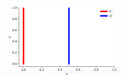
  所以有如下距离定义，只有当 $\theta=0$时，才能达到最小，但是除了 $W$，均达不到最下值。：
  $\begin{aligned} W(\mathbb{P}_{0},\mathbb{P}_{\theta})&=|\theta|\\ \mathbf{JS}(\mathbb{P}_{0},\mathbb{P}_{\theta})&= \begin{cases} \log 2& \text{if $\theta \neq$0}\\ 0& \text{if $\theta=$0} \end{cases} \\ \mathbf{KL}(\mathbb{P}_{0},\mathbb{P}_{\theta})&=\mathbf{KL}(\mathbb{P}_{\theta},\mathbb{P}_{0})= \begin{cases} \infty& \text{if $\theta \neq$0}\\ 0& \text{if $\theta=$0} \end{cases} \\ \mathbf{TV}(\mathbb{P}_{0},\mathbb{P}_{\theta})&= \begin{cases} 1 & \text{if $\theta \neq$0}\\ 0& \text{if $\theta=$0} \end{cases} \\ \text{where: $D_{KL}(P \| Q$) }& \text{$= \sum_{x=0, y \sim U(0, 1)} 1 \cdot \log\frac{1}{0} = +\infty$ } \\ \text{ $D_{JS}(P \| Q$)}&= \text{$\frac{1}{2}(\sum_{x=0, y \sim U(0, 1)} 1 \cdot \log\frac{1}{1/2} + \sum_{x=0, y \sim U(0, 1)} 1 \cdot \log\frac{1}{1/2}) = \log 2$ } \\ \tag{3} \end{aligned}$

• Why Wasserstein is indeed weak?（有待研究更新）
  论文还叙述了为什么Wasserstein距离是比 $\mathbf{JS}$距离差的，但作者仍然用Wasserstein距离。证明用到了一些泛函的概念。 $\mathcal{X}$为 $\mathbb{R}^2$中的一组集，即 $\mathcal{X}\in \mathbb{R}^2$； $C_b(\mathcal{X})$是将 $\mathcal{X}$映射到 $\mathbb{R}$的函数的空间（ $C_b(\mathcal{X})$中每一个元素都是函数，它是一集合）：
  $\begin{aligned} C_b(\mathcal{X}) &= \{ f:\mathcal{X} \rightarrow \mathbb{R}, &\text{$f$ is continuous and bounded} \}\\ \tag{4} \end{aligned}$
  当有 $f \in C_b(\mathcal{X})$后，按照矩阵的方式理解则有，所以 $f$的无穷范数即是得到的 $\mathbb{R}^2$空间结果的绝对值最大值：
  $\begin{aligned} \text{assume:}f_{m \times n} \cdot \mathcal{X}_{n \times 1}= \mathbb{R}_{m \times 1} \\ \therefore f_{m \times n} \cdot \mathcal{X}_{n \times d}= \mathbb{R}_{m \times d} \\ \therefore \|f\|_{\infin} = \max_{x \in \mathcal{X}}|f(x)| \tag{5} \end{aligned}$
  给集合 $(C_b(\mathcal{X})$赋予一范数进行约束得到一个赋范向量空间 $(C_b(\mathcal{X}),\| \cdot \| )$（ $f_\infin$范数诱导的自然拓扑）
  $\begin{aligned} {\mathbb {E}}\times {\mathbb {E}}\longrightarrow {\mathbb {R}} {\displaystyle \ (x,y)\mapsto \Vert x-y\Vert } \ (x,y)\mapsto \Vert x-y\Vert \tag{6} \end{aligned}$

3.WGAN

• 利用Kantorovich-Rubinstein对偶性，将推土距离转换如下（but why?有待研究更新），其中 $K$代表 $\text{K-Lipschitz}:\lvert f(x_1) - f(x_2) \rvert \leq K \lvert x_1 - x_2 \rvert$，约束函数平稳，斜率不能太大：
  $\begin{aligned} W(\mathbb{P}_{r},\mathbb{P}_{\theta})= \frac{1}{K} \sup_{\| f \|_L \leq K} \mathbb{E}_{x \sim \mathbb{P}_{r}}[f(x)] - \mathbb{E}_{x \sim \mathbb{P}_{\theta}}[f(x)] \tag{7} \end{aligned}$
  所以有 $\text{K-Lipschitz}$函数 $\{ f_w \}_{w \in W}$，判别器需要学到一个好的 $f$，并且要求损失函数如下进行收敛：
  $\begin{aligned} L(\mathbb{P}_{r},\mathbb{P}_{\theta})=W(\mathbb{P}_{r},\mathbb{P}_{\theta})= \max_{w \in W} \mathbb{E}_{x \sim p_r}[f_w(x)] - \mathbb{E}_{z \sim p_r(z)}[f_w(g_\theta(z))] \tag{8} \end{aligned}$
  

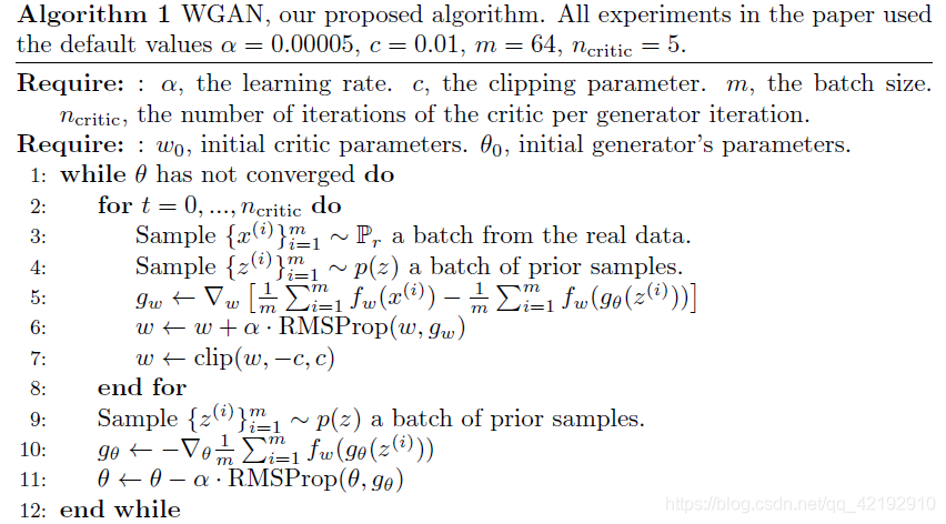
正如算法流程所述， 以便使用梯度下降，所以文中使用约束权重范围的方法，以防止改变权重造成很大的改变，确保 $\text{1-Lipschitz}$。

4.WGAN-GP

Intro

• 在WGAN-GP的文章中提出了使用权重约束的问题，会不收敛或者仅产生较差的样本。but sometimes can still generate only poor samples or fail to converge.
• 提出了新的裁剪权重的方法（梯度惩罚gradient penalty）。We propose an alternative to clipping weights: penalize the norm of gradient of the critic with respect to its input.

Details

• 对于 $\text{1-Lipschitz}$的函数 $f$意味这 $\mathbb{P}_{r},\mathbb{P}_{\theta}$之间的梯度不会超过1，所以惩罚梯度的意思就是惩罚大于1的情况。所以损失就如下改变：
  $\begin{aligned} L=\mathbb{E}_{\widetilde{x} \sim \mathbb{P}_{\theta}} \left[D(\widetilde{x})\right]-\mathbb{E}_{\widetilde{x} \sim \mathbb{P}_{r}} \left[D(\widetilde{x})\right] + \lambda \mathbb{E}_{\hat{x} \sim \mathbb{P}_{\hat{x}}} \left[ (\| \bigtriangledown_{\hat{x}}D(\hat{x}) \|_2-1)^2 \right] \tag{9} \end{aligned}$
  前一部分很容易理解即是GAN的标准损失，后面一项就是超参数 $\lambda$下对梯度进行约束的表达。
• 由上述式子理应该对所有的数据进行惩罚，但是这样却很棘手，无法对所有的数据都保证斜率小于1，所以是重新随机抽出一个数据集 $\hat{x}$，仅对其进行惩罚。
• 没有BN层， $\lambda$设置为10。
• 理论上惩罚应该仅仅对所有的大于1，而小于1的部分不用管 $\max\{0 \text{ , } (\| \bigtriangledown_{\hat{x}}D(\hat{x}) \|_2-1)^2 \}$，但是让其靠近1理论上更好。We encourage the norm of the gradient to go towards 1 (two-sided penalty) instead of just staying below 1 (one-sided penalty).