跟着Leo机器学习实战：sklearn笔记--线性模型

跟着Leo机器学习实战：sklearn笔记

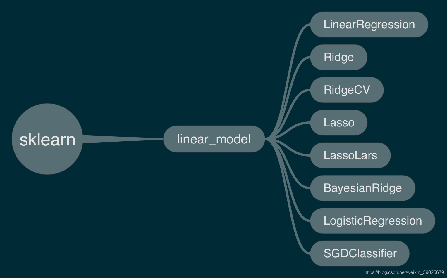
sklearn框架–线性模型

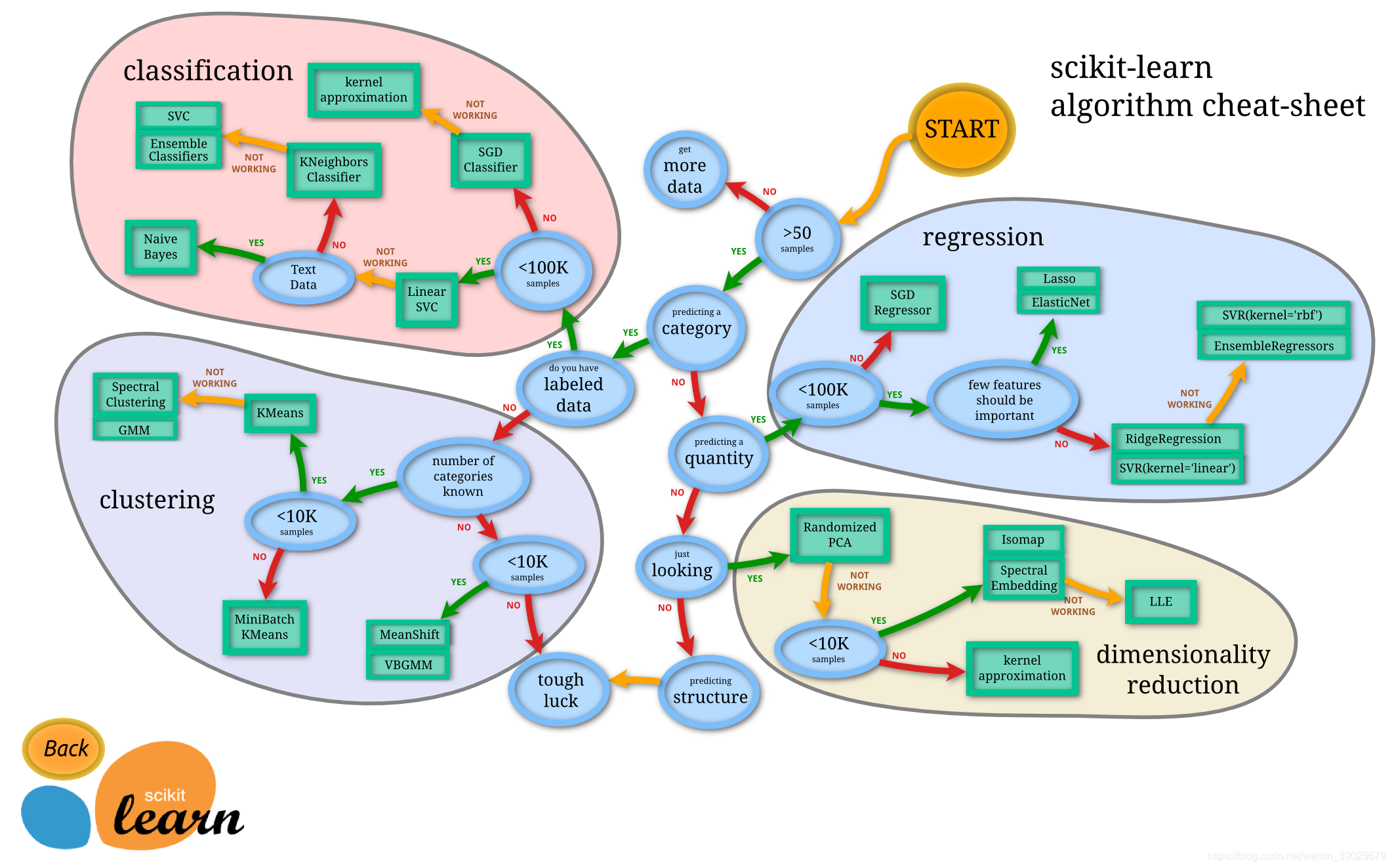
一般机器学习流程

Supervised learning监督学习

线性模型

每一个模型都有一个拟合函数和预测函数

fit()
predict()

Ordinary Least Squares

from sklearn import linear_model
reg = linear_model.LinearRegression()
reg.fit([[0, 0], [1, 1], [2, 2]], [0, 1, 2])

reg.coef_

Ridge regression and classification

from sklearn import linear_model
reg = linear_model.Ridge(alpha=.5)
reg.fit([[0, 0], [0, 0], [1, 1]], [0, .1, 1])

reg.coef_

reg.intercept_

Setting the regularization parameter: generalized Cross-Validation

import numpy as np
from sklearn import linear_model
reg = linear_model.RidgeCV(alphas=np.logspace(-6, 6, 13))
reg.fit([[0, 0], [0, 0], [1, 1]], [0, .1, 1])


reg.alpha_

Lasso

from sklearn import linear_model
reg = linear_model.Lasso(alpha=0.1)
reg.fit([[0, 0], [1, 1]], [0, 1])

reg.predict([[1, 1]])

LARS Lasso

from sklearn import linear_model
reg = linear_model.LassoLars(alpha=.1)
reg.fit([[0, 0], [1, 1]], [0, 1])

reg.coef_

Bayesian Ridge Regression

from sklearn import linear_model
X = [[0., 0.], [1., 1.], [2., 2.], [3., 3.]]
Y = [0., 1., 2., 3.]
reg = linear_model.BayesianRidge()
reg.fit(X, Y)

Logistic regression

MNIST classification using multinomial logistic + L1

import time
import matplotlib.pyplot as plt
import numpy as np

from sklearn.datasets import fetch_openml
from sklearn.linear_model import LogisticRegression
from sklearn.model_selection import train_test_split
from sklearn.preprocessing import StandardScaler
from sklearn.utils import check_random_state

print(__doc__)

# Author: Arthur Mensch <[email protected]>
# License: BSD 3 clause

# Turn down for faster convergence
t0 = time.time()
train_samples = 5000

# Load data from https://www.openml.org/d/554
X, y = fetch_openml('mnist_784', version=1, return_X_y=True)

random_state = check_random_state(0)
permutation = random_state.permutation(X.shape[0])
X = X[permutation]
y = y[permutation]
X = X.reshape((X.shape[0], -1))

X_train, X_test, y_train, y_test = train_test_split(
    X, y, train_size=train_samples, test_size=10000)

scaler = StandardScaler()
X_train = scaler.fit_transform(X_train)
X_test = scaler.transform(X_test)

# Turn up tolerance for faster convergence
clf = LogisticRegression(
    C=50. / train_samples, penalty='l1', solver='saga', tol=0.1
)#实例化Logistic回归模型
clf.fit(X_train, y_train)#进行训练
sparsity = np.mean(clf.coef_ == 0) * 100
score = clf.score(X_test, y_test)#评估模型
# print('Best C % .4f' % clf.C_)
print("Sparsity with L1 penalty: %.2f%%" % sparsity)
print("Test score with L1 penalty: %.4f" % score)

coef = clf.coef_.copy()
plt.figure(figsize=(10, 5))
scale = np.abs(coef).max()
for i in range(10):
    l1_plot = plt.subplot(2, 5, i + 1)
    l1_plot.imshow(coef[i].reshape(28, 28), interpolation='nearest',
                   cmap=plt.cm.RdBu, vmin=-scale, vmax=scale)
    l1_plot.set_xticks(())
    l1_plot.set_yticks(())
    l1_plot.set_xlabel('Class %i' % i)
plt.suptitle('Classification vector for...')

run_time = time.time() - t0
print('Example run in %.3f s' % run_time)
plt.show()

提取处最重要的训练函数

clf = LogisticRegression(
    C=50. / train_samples, penalty='l1', solver='saga', tol=0.1
)#实例化Logistic回归模型
clf.fit(X_train, y_train)#进行训练
sparsity = np.mean(clf.coef_ == 0) * 100
score = clf.score(X_test, y_test)#评估模型

Stochastic Gradient Descent - SGD

Classification

from sklearn.linear_model import SGDClassifier
X = [[0., 0.], [1., 1.]]
y = [0, 1]
clf = SGDClassifier(loss="hinge", penalty="l2", max_iter=5)
clf.fit(X, y)

其他参数选择
loss=“hinge”: (soft-margin) linear Support Vector Machine,
loss=“modified_huber”: smoothed hinge loss,
loss=“log”: logistic regression,

预测

clf.predict([[2., 2.]])

模型参数

clf.coef_

Regression

loss=“squared_loss”: Ordinary least squares,
loss=“huber”: Huber loss for robust regression,
loss=“epsilon_insensitive”: linear Support Vector Regression.