【数据分析4】scikit-learn机器学习

1.机器学习方法：

• 构造间隔理论分布：聚类分析和模式识别
• 人工神经网络
• 决策树
• 感知器
• 支持向量机
• 集成学习AdaBoos
• 降维与度量学习
• 聚类
• 贝叶斯分类器

• 构造条件概率：回归分析和统计分类
• 高斯过程回归
• 线性判别分析
• 最近邻居法
• 径向基函数核

• 通过再生模型构造概率密度函数：
• 最大期望算法
• 概率图模型：包括贝叶斯网和 Markov随机场
• Generative Topographic Mapping

• 近似推断技术：
• 马尔可夫链
• 蒙特卡罗方法
• 变分法

• 最优化：大多数以上方法，直接或者间接 使用最优化算法。

**

2.常见机器学习任务

2.1有监督学习（有标准答案）

如：1万张图片，5千猫，5千狗，训练机器识别，
再之后机器就能自动识别猫狗

分类 识别某个对象属于哪个类别

样本属于两个或更多个类，我们想从已经标
记的数据中学习如何预测未标记数据的类别。

• 应用: 垃圾邮件检测， 图像识别
• 算法: SVM, nearest neighbors, random forest

归为离散问题

回归 预测与对象相关联的连续值属性
• 应用: 药物反应，股价
• 算法: SVR, ridge regression, Lasso

如果期望的输出由一个或多个连续变量组成，
则该任务称为回归 。

归为连续问题

2.2无监督学习（无标准答案）

给你1万照片，包括狗和猫，机器自己去识别并按照属性分类

聚类 将相似对象自动分组
• 应用: 客户细分，分组 实验结果
• 算法: kMeans, spectral clustering, meanshift

训练数据由没有任何相应目标值的一组输入
组成，目标是把相似的对象通过分类的方法
分成不同的组别。

3.scikit_learn简介

官网地址： http://scikit-learn.org/
中文文档地址： http://sklearn.apachecn.org/

3.1安装模块

Windows：pip install scikit_learn
Mac：pip3 install scikit_learn

3.2模块简介

除了能够实现分类，回归，聚类还可以实现
降维
减少要考虑的随机变量的数量
• 应用: 可视化，提高效率
• 算法: PCA, feature selection, nonnegative matrix factorization
如数据包含姓名，性别，体重，籍贯，一家几口人，预测每个人的身高，这几个数据对于升高的影响不同，且姓名对于身高没有影响，籍贯和一家几口人影响较小，我们可以去掉姓名这个维度，并将籍贯和一家几口合并为一个维度，实现降维。
模型选择
比较，验证，选择参数和模型
• 目标: 通过参数调整提 高精度
• 模型: grid search, cross validation, metrics
预处理 特征提取和归一化
• 应用: 把输入数据（如 文本）转换为机器学习 算法可用的数据
• 算法: preprocessing, feature extraction

3.4入门练习

鸢尾花分类任务
数据描述：
• scikit-learn自带数据
• 根据花瓣的长宽，茎的长宽四个数据
• 对该花朵进行分类，共三种类型

3.4.1 导入模块查看数据

from sklearn import datasets   #注意scikit-learn在Python中是sklearn

iris = datasets.load_iris()    #直接load_iris()即可获取自带数据
print(iris)

{'data': array([[5.1, 3.5, 1.4, 0.2],
       [4.9, 3. , 1.4, 0.2],
       [4.7, 3.2, 1.3, 0.2],
       [4.6, 3.1, 1.5, 0.2],
       [5. , 3.6, 1.4, 0.2],
       [5.4, 3.9, 1.7, 0.4],
       [4.6, 3.4, 1.4, 0.3],
       [5. , 3.4, 1.5, 0.2],
       [4.4, 2.9, 1.4, 0.2],
       [4.9, 3.1, 1.5, 0.1],
       [5.4, 3.7, 1.5, 0.2],
       [4.8, 3.4, 1.6, 0.2],
       [4.8, 3. , 1.4, 0.1],
       [4.3, 3. , 1.1, 0.1],
       [5.8, 4. , 1.2, 0.2],
       [5.7, 4.4, 1.5, 0.4],
       [5.4, 3.9, 1.3, 0.4],
       [5.1, 3.5, 1.4, 0.3],
       [5.7, 3.8, 1.7, 0.3],
       [5.1, 3.8, 1.5, 0.3],
       [5.4, 3.4, 1.7, 0.2],
       [5.1, 3.7, 1.5, 0.4],
       [4.6, 3.6, 1. , 0.2],
       [5.1, 3.3, 1.7, 0.5],
       [4.8, 3.4, 1.9, 0.2],
       [5. , 3. , 1.6, 0.2],
       [5. , 3.4, 1.6, 0.4],
       [5.2, 3.5, 1.5, 0.2],
       [5.2, 3.4, 1.4, 0.2],
       [4.7, 3.2, 1.6, 0.2],
       [4.8, 3.1, 1.6, 0.2],
       [5.4, 3.4, 1.5, 0.4],
       [5.2, 4.1, 1.5, 0.1],
       [5.5, 4.2, 1.4, 0.2],
       [4.9, 3.1, 1.5, 0.2],
       [5. , 3.2, 1.2, 0.2],
       [5.5, 3.5, 1.3, 0.2],
       [4.9, 3.6, 1.4, 0.1],
       [4.4, 3. , 1.3, 0.2],
       [5.1, 3.4, 1.5, 0.2],
       [5. , 3.5, 1.3, 0.3],
       [4.5, 2.3, 1.3, 0.3],
       [4.4, 3.2, 1.3, 0.2],
       [5. , 3.5, 1.6, 0.6],
       [5.1, 3.8, 1.9, 0.4],
       [4.8, 3. , 1.4, 0.3],
       [5.1, 3.8, 1.6, 0.2],
       [4.6, 3.2, 1.4, 0.2],
       [5.3, 3.7, 1.5, 0.2],
       [5. , 3.3, 1.4, 0.2],
       [7. , 3.2, 4.7, 1.4],
       [6.4, 3.2, 4.5, 1.5],
       [6.9, 3.1, 4.9, 1.5],
       [5.5, 2.3, 4. , 1.3],
       [6.5, 2.8, 4.6, 1.5],
       [5.7, 2.8, 4.5, 1.3],
       [6.3, 3.3, 4.7, 1.6],
       [4.9, 2.4, 3.3, 1. ],
       [6.6, 2.9, 4.6, 1.3],
       [5.2, 2.7, 3.9, 1.4],
       [5. , 2. , 3.5, 1. ],
       [5.9, 3. , 4.2, 1.5],
       [6. , 2.2, 4. , 1. ],
       [6.1, 2.9, 4.7, 1.4],
       [5.6, 2.9, 3.6, 1.3],
       [6.7, 3.1, 4.4, 1.4],
       [5.6, 3. , 4.5, 1.5],
       [5.8, 2.7, 4.1, 1. ],
       [6.2, 2.2, 4.5, 1.5],
       [5.6, 2.5, 3.9, 1.1],
       [5.9, 3.2, 4.8, 1.8],
       [6.1, 2.8, 4. , 1.3],
       [6.3, 2.5, 4.9, 1.5],
       [6.1, 2.8, 4.7, 1.2],
       [6.4, 2.9, 4.3, 1.3],
       [6.6, 3. , 4.4, 1.4],
       [6.8, 2.8, 4.8, 1.4],
       [6.7, 3. , 5. , 1.7],
       [6. , 2.9, 4.5, 1.5],
       [5.7, 2.6, 3.5, 1. ],
       [5.5, 2.4, 3.8, 1.1],
       [5.5, 2.4, 3.7, 1. ],
       [5.8, 2.7, 3.9, 1.2],
       [6. , 2.7, 5.1, 1.6],
       [5.4, 3. , 4.5, 1.5],
       [6. , 3.4, 4.5, 1.6],
       [6.7, 3.1, 4.7, 1.5],
       [6.3, 2.3, 4.4, 1.3],
       [5.6, 3. , 4.1, 1.3],
       [5.5, 2.5, 4. , 1.3],
       [5.5, 2.6, 4.4, 1.2],
       [6.1, 3. , 4.6, 1.4],
       [5.8, 2.6, 4. , 1.2],
       [5. , 2.3, 3.3, 1. ],
       [5.6, 2.7, 4.2, 1.3],
       [5.7, 3. , 4.2, 1.2],
       [5.7, 2.9, 4.2, 1.3],
       [6.2, 2.9, 4.3, 1.3],
       [5.1, 2.5, 3. , 1.1],
       [5.7, 2.8, 4.1, 1.3],
       [6.3, 3.3, 6. , 2.5],
       [5.8, 2.7, 5.1, 1.9],
       [7.1, 3. , 5.9, 2.1],
       [6.3, 2.9, 5.6, 1.8],
       [6.5, 3. , 5.8, 2.2],
       [7.6, 3. , 6.6, 2.1],
       [4.9, 2.5, 4.5, 1.7],
       [7.3, 2.9, 6.3, 1.8],
       [6.7, 2.5, 5.8, 1.8],
       [7.2, 3.6, 6.1, 2.5],
       [6.5, 3.2, 5.1, 2. ],
       [6.4, 2.7, 5.3, 1.9],
       [6.8, 3. , 5.5, 2.1],
       [5.7, 2.5, 5. , 2. ],
       [5.8, 2.8, 5.1, 2.4],
       [6.4, 3.2, 5.3, 2.3],
       [6.5, 3. , 5.5, 1.8],
       [7.7, 3.8, 6.7, 2.2],
       [7.7, 2.6, 6.9, 2.3],
       [6. , 2.2, 5. , 1.5],
       [6.9, 3.2, 5.7, 2.3],
       [5.6, 2.8, 4.9, 2. ],
       [7.7, 2.8, 6.7, 2. ],
       [6.3, 2.7, 4.9, 1.8],
       [6.7, 3.3, 5.7, 2.1],
       [7.2, 3.2, 6. , 1.8],
       [6.2, 2.8, 4.8, 1.8],
       [6.1, 3. , 4.9, 1.8],
       [6.4, 2.8, 5.6, 2.1],
       [7.2, 3. , 5.8, 1.6],
       [7.4, 2.8, 6.1, 1.9],
       [7.9, 3.8, 6.4, 2. ],
       [6.4, 2.8, 5.6, 2.2],
       [6.3, 2.8, 5.1, 1.5],
       [6.1, 2.6, 5.6, 1.4],
       [7.7, 3. , 6.1, 2.3],
       [6.3, 3.4, 5.6, 2.4],
       [6.4, 3.1, 5.5, 1.8],
       [6. , 3. , 4.8, 1.8],
       [6.9, 3.1, 5.4, 2.1],
       [6.7, 3.1, 5.6, 2.4],
       [6.9, 3.1, 5.1, 2.3],
       [5.8, 2.7, 5.1, 1.9],
       [6.8, 3.2, 5.9, 2.3],
       [6.7, 3.3, 5.7, 2.5],
       [6.7, 3. , 5.2, 2.3],
       [6.3, 2.5, 5. , 1.9],
       [6.5, 3. , 5.2, 2. ],
       [6.2, 3.4, 5.4, 2.3],
       [5.9, 3. , 5.1, 1.8]]), 'target': array([0, 0, 0, 0, 0, 0, 0, 0, 0, 0, 0, 0, 0, 0, 0, 0, 0, 0, 0, 0, 0, 0,
       0, 0, 0, 0, 0, 0, 0, 0, 0, 0, 0, 0, 0, 0, 0, 0, 0, 0, 0, 0, 0, 0,
       0, 0, 0, 0, 0, 0, 1, 1, 1, 1, 1, 1, 1, 1, 1, 1, 1, 1, 1, 1, 1, 1,
       1, 1, 1, 1, 1, 1, 1, 1, 1, 1, 1, 1, 1, 1, 1, 1, 1, 1, 1, 1, 1, 1,
       1, 1, 1, 1, 1, 1, 1, 1, 1, 1, 1, 1, 2, 2, 2, 2, 2, 2, 2, 2, 2, 2,
       2, 2, 2, 2, 2, 2, 2, 2, 2, 2, 2, 2, 2, 2, 2, 2, 2, 2, 2, 2, 2, 2,
       2, 2, 2, 2, 2, 2, 2, 2, 2, 2, 2, 2, 2, 2, 2, 2, 2, 2]), 'target_names': array(['setosa', 'versicolor', 'virginica'], dtype='<U10'), 'DESCR': '.. _iris_dataset:\n\nIris plants dataset\n--------------------\n\n**Data Set Characteristics:**\n\n    :Number of Instances: 150 (50 in each of three classes)\n    :Number of Attributes: 4 numeric, predictive attributes and the class\n    :Attribute Information:\n        - sepal length in cm\n        - sepal width in cm\n        - petal length in cm\n        - petal width in cm\n        - class:\n                - Iris-Setosa\n                - Iris-Versicolour\n                - Iris-Virginica\n                \n    :Summary Statistics:\n\n    ============== ==== ==== ======= ===== ====================\n                    Min  Max   Mean    SD   Class Correlation\n    ============== ==== ==== ======= ===== ====================\n    sepal length:   4.3  7.9   5.84   0.83    0.7826\n    sepal width:    2.0  4.4   3.05   0.43   -0.4194\n    petal length:   1.0  6.9   3.76   1.76    0.9490  (high!)\n    petal width:    0.1  2.5   1.20   0.76    0.9565  (high!)\n    ============== ==== ==== ======= ===== ====================\n\n    :Missing Attribute Values: None\n    :Class Distribution: 33.3% for each of 3 classes.\n    :Creator: R.A. Fisher\n    :Donor: Michael Marshall (MARSHALL%[email protected])\n    :Date: July, 1988\n\nThe famous Iris database, first used by Sir R.A. Fisher. The dataset is taken\nfrom Fisher\'s paper. Note that it\'s the same as in R, but not as in the UCI\nMachine Learning Repository, which has two wrong data points.\n\nThis is perhaps the best known database to be found in the\npattern recognition literature.  Fisher\'s paper is a classic in the field and\nis referenced frequently to this day.  (See Duda & Hart, for example.)  The\ndata set contains 3 classes of 50 instances each, where each class refers to a\ntype of iris plant.  One class is linearly separable from the other 2; the\nlatter are NOT linearly separable from each other.\n\n.. topic:: References\n\n   - Fisher, R.A. "The use of multiple measurements in taxonomic problems"\n     Annual Eugenics, 7, Part II, 179-188 (1936); also in "Contributions to\n     Mathematical Statistics" (John Wiley, NY, 1950).\n   - Duda, R.O., & Hart, P.E. (1973) Pattern Classification and Scene Analysis.\n     (Q327.D83) John Wiley & Sons.  ISBN 0-471-22361-1.  See page 218.\n   - Dasarathy, B.V. (1980) "Nosing Around the Neighborhood: A New System\n     Structure and Classification Rule for Recognition in Partially Exposed\n     Environments".  IEEE Transactions on Pattern Analysis and Machine\n     Intelligence, Vol. PAMI-2, No. 1, 67-71.\n   - Gates, G.W. (1972) "The Reduced Nearest Neighbor Rule".  IEEE Transactions\n     on Information Theory, May 1972, 431-433.\n   - See also: 1988 MLC Proceedings, 54-64.  Cheeseman et al"s AUTOCLASS II\n     conceptual clustering system finds 3 classes in the data.\n   - Many, many more ...', 'feature_names': ['sepal length (cm)', 'sepal width (cm)', 'petal length (cm)', 'petal width (cm)'], 'filename': 'C:\\Users\\lenovo\\AppData\\Local\\Programs\\Python\\Python37\\lib\\site-packages\\sklearn\\datasets\\data\\iris.csv'}

3.4.2 算法svc

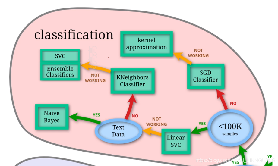
因为我们要实现分类，且数据小于100k，选择LinearSVC
LinearSVC是SVM的一种

我们导入模块完善代码：
1.数据切分

from sklearn import datasets   #注意scikit-learn在Python中是sklearn

from sklearn import svm        #LinearSVC是SVM的一种
from sklearn.model_selection import train_test_split   
#train_test_split可以将数据分为两个部分
#一部分为train，即训练用数据 一部分为test，即测试用数据

 
iris = datasets.load_iris()    #直接load_iris()即可获取自带数据
x = iris.data
y = iris.target
x_train,x_test,y_train,y_test = train_test_split(X,y,test_size=0.3,random_state=0) 
 #test_size可以调节训练和测试数据比例 random_state可以确保切分状态一致

2.数据训练
通用流程：

1. 创建分类器/回归器等
2. XXX.fit(训练数据输入值，对应的正确结果)
3. XXX.predict(待检测数据输入值)

#创建一个LinearSVC分类器  
clf = svm.LinearSVC()
clf.fit(X_train,y_train)

3.模型得分

print("score:{}".format(clf.score(X_test,y_test)))  #通过.score()计算模型得分

score:0.9333333333333333

4.模型预测

y_predict = clf.predict(X_test)                     #通过.predict()预测新数
print(y_predict)
print(y_test)

[2 1 0 2 0 2 0 1 1 1 2 1 1 1 1 0 1 1 0 0 2 2 0 0 2 0 0 1 1 0 2 2 0 2 2 1 0
 2 1 1 2 0 2 0 0]
[2 1 0 2 0 2 0 1 1 1 2 1 1 1 1 0 1 1 0 0 2 1 0 0 2 0 0 1 1 0 2 1 0 2 2 1 0
 1 1 1 2 0 2 0 0]

3.5小练习

波士顿房价预测任务
数据描述：
• scikit-learn自带数据
• 总共有506个数据
• 共有13个属性
• 需要预测房价
1.获取并切分数据

from sklearn import datasets 
from sklearn.model_selection import train_test_split 

boston = datasets.load_boston()   #获取数据


X = boston.data
y = boston.target                #正确答案
X_train,X_test,y_train,y_test = train_test_split(X,y,test_size=0.3,random_state=13)

数据属性说明：
数据属性说明
CRIM 城镇人均犯罪率
ZN 占地面积超过2.5万平方英尺的住宅用地比例
INDUS 城镇非零售业务地区的比例 CHAS 查尔斯河虚拟变量 (= 1 如果土地在河边；否则是0)
NOX 一氧化氮浓度（每1000万份）
RM 平均每居民房数
AGE 在1940年之前建成的所有者占用单位的比例
DIS 与五个波士顿就业中心的加权距离
RAD 辐射状公路的可达性指数
TAX 每10,000美元的全额物业税率
PTRATIO 城镇师生比例
B 1000(Bk - 0.63)^2 其中 Bk 是城镇的黑人比例
LSTAT 人口中地位较低人群的百分数

2.该问题为回归问题：

样本数小于100k，且应该是有几个数据比较重要，故选择lasso

from sklearn import datasets 
from sklearn import linear_model
from sklearn.model_selection import train_test_split 

boston = datasets.load_boston()   #获取数据


X = boston.data
y = boston.target                #正确答案
X_train,X_test,y_train,y_test = train_test_split(X,y,test_size=0.3,random_state=13)

lasso = linear_model.Lasso()
lasso.fit(X_train,y_train)

3.评价得分

from sklearn import datasets 
from sklearn import linear_model
from sklearn.model_selection import train_test_split 
from sklearn.metrics import mean_squared_error              #均方差

boston = datasets.load_boston()   #获取数据


X = boston.data
y = boston.target                #正确答案
X_train,X_test,y_train,y_test = train_test_split(X,y,test_size=0.3,random_state=13)

lasso = linear_model.Lasso()
lasso.fit(X_train,y_train)

mse = mean_squared_error(y_test,lasso.predict(X_test))
score = lasso.score(X_test,y_test)
print('MSE:{}'.format(mse))
print("Score:{}".format(score))

MSE:29.421277284405665
Score:0.6438186963381397

结果说明勉强好于瞎猜

4.调节参数
设置Lasso的参数alpha

lasso = linear_model.Lasso(alpha=0.1)

MSE:25.002006756302062
Score:0.697319484992502

结果说明确实准确率有所提升
5.GridSearchCV 网格搜索测试

from sklearn import datasets 
from sklearn import linear_model
from sklearn.model_selection import train_test_split 
from sklearn.metrics import mean_squared_error              #均方差
import numpy as np
from sklearn.model_selection import GridSearchCV            #利用scikit-learn的网格搜索调节参数

boston = datasets.load_boston()   #获取数据


X = boston.data
y = boston.target                #正确答案
X_train,X_test,y_train,y_test = train_test_split(X,y,test_size=0.3,random_state=13)

alpha_range = np.arange(0,1,0.05)  #list
param_grid = {"alpha":alpha_range}  #创建字典
lasso = linear_model.Lasso()
lasso_search = GridSearchCV(lasso,param_grid)
lasso_search.fit(X_train,y_train)
for result in lasso_search.cv_results_:
	print(result,lasso_search.cv_results_[result])
print(lasso_search.best_score_)
print(lasso_search.best_params_)
print(lasso_search.best_estimator_)

当然也可以应用于其他模型：

'''eln_reg = linear_model.ElasticNet()   #其他模型
svr_reg = svm.SVR()
nusver_reg = svm.NuSVR()
ridge_reg = linear_model.Ridge()
gbr_reg = ensemble.GradientBoostiingRegressor()
'''

6.RandomizedSearchCV 随机搜索
利用随机搜索可以降低搜索复杂度
两种方法对比：

a）目标函数为 f(x,y)=g(x)+h(y)，其中绿色为g(x),黄色为h(y)，目的是求f的最大值。
（b）其中由于g(x)数值上要明显大于h(y)，因此有f(x,y)=g(x)+h(y)≈g(x)，也就是说在整体求解f(x,y)最大值的过程中，g(x)的影响明显大于h(y)。
（c）两个图都进行9次实验（搜索），可以看到左图实际探索了各三个点（在横轴和纵轴上的投影均为3个），而右图探索了9个不同的点（横轴纵轴均是，不过实际上横轴影响更大）。
（d）右图更可能找到目标函数的最大值。
因此引入随机因素在某些情况下可以提高寻优效率。```python
n_estimators_range = np.arange(10,1000,10)
max_depth_range = np.arange(1,10)
learning_rate_range = [0.001,0.01,0.1]
param_grid = {
“n_estimators”:n_estimators_range,
“max_depth”:max_depth_range,
“learning_rate”:learning_rate_range
}
gbr_search =RandomizedSearchCV(gbr_reg,param_grid,n_iter=50) #注意添加n_iter=测试次数确定需要测试的次数
gbr_search.fit(X_train,y_train)
for result in gbr_search.grid_scores_:
print(result)
print(gbr_search.best_score_)
print(gbr_search.best_params_)
print(gbr_search.best_estimator_)

后续将会持续更新excel，ppt，爬虫，人工智能等相关内容，敬请关注