04_TrainingModels_03

04_TrainingModels_Normal Equation(正态方程,正规方程) Derivation_Gradient Descent_Polynomial Regression:
https://blog.csdn.net/Linli522362242/article/details/104005906

04_TrainingModels_02_regularization_Ridge_Lasso_Elastic Net_Early Stopping:
https://blog.csdn.net/Linli522362242/article/details/104070847

sklearn.linear_model.LogisticRegression
https://scikit-learn.org/stable/modules/generated/sklearn.linear_model.LogisticRegression.html
The ‘newton-cg’, ‘sag’, and ‘lbfgs’ solvers support only L2 regularization (==, ==)with primal formulation, or no regularization. The ‘liblinear’ solver supports both L1 and L2 regularization, with a dual formulation only for the L2 penalty. The Elastic-Net regularization is only supported by the ‘saga’ solver.

solver{‘newton-cg’, ‘lbfgs’, ‘liblinear’, ‘sag’, ‘saga’}, default=’lbfgs’

Algorithm to use in the optimization problem.

For small datasets, ‘liblinear’ is a good choice, whereas ‘sag’ and ‘saga’ are faster for large ones.
For multiclass problems, only ‘newton-cg’, ‘sag’, ‘saga’ and ‘lbfgs’ handle multinomial loss; ‘liblinear’ is limited to one-versus-rest schemes.
‘newton-cg’, ‘lbfgs’, ‘sag’ and ‘saga’ handle L2 or no penalty
‘liblinear’ and ‘saga’ also handle L1 penalty
‘saga’ also supports ‘elasticnet’ penalty
‘liblinear’ does not support setting penalty='none'

Note that ‘sag’ and ‘saga’ fast convergence is only guaranteed on features with approximately the same scale. You can preprocess the data with a scaler from sklearn.preprocessing.

However, having a good understanding of how things work can help you quickly home找到 in on the appropriate model, the right training algorithm to use, and a good set of hyperparameters for your task. Understanding what’s under the hood黑箱子内部 will also help you debug issues and perform error analysis more efficiently.

Using a direct “closed-form” equation that directly computes the model parameters that best fit the model to the training set (i.e., the model parameters that minimize the cost function over the training set).

We will replace our hypothesis in error function(MSE cost function). ( weight w ==

)

solve Normal Equation( has a closed-form solution) ==> find the value of θ ==> minimizes MSE cost function ==> minimizes the RMSE

X = 2 * np.random.rand(100, 1)
y = 4 + 3*X + np.random.randn(100,1) # np.random.randn(100,1) == Gaussian noise 
theta_best = np.linalg.inv( X_b.T.dot((X_b)) ).dot(X_b.T).dot(y)
theta_best

X_new = np.array([[0], [2]])
X_new_b = np.c_[np.ones((2,1)), X_new
               ]# add x0 =1 to each in each instance
X_new_b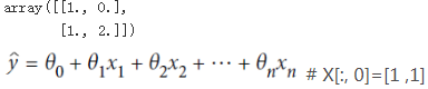

y_predict = X_new_b.dot(theta_best)
y_predict

# 4.11097362*1 + 2.87496178*0= 4.11097362

Using an iterative optimization approach, called Gradient Descent梯度下降 (GD), that gradually tweaks the model parameters to minimize the cost function over the training set, eventually converging收敛 to the same set of parameters as the first method.

*1 and
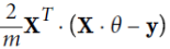
Equation 4-6. Gradient vector of the cost function ()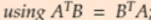
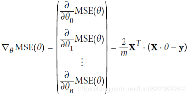Note: X is x0==1, x1, x2, ..., xn

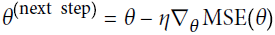
Equation 4-7. Gradient Descent step

batch gradient descent
```
eta = 0.1 # learning rate
n_iterations = 1000
m=100
 
theta = np.random.randn(2,1) # random initialization
 
for iteration in range(n_iterations):
    gradients = 2/m * X_b.T.dot( X_b.dot(theta) - y )
    theta = theta - eta*gradients
    
theta #lin_reg.intercept_, lin_reg.coef_  #theta_best
```
```
X_new_b.dot(theta) #predictions
```
1. the learning rate is too low: the algorithm will eventually reach the solution, but it will take a long time
2. the learning rate is too high: the algorithm diverges发散的, jumping all over the place and actually getting further and further away from the solution at every step.
To find a good learning rate, you can use grid search (see https://blog.csdn.net/Linli522362242/article/details/103646927). However, you may want to limit the number of iterations so that grid search can eliminate models(kernel) that take too long to converge.
You may wonder how to set the number of iterations. If it is too low, you will still be far away from the optimal solution when the algorithm stops, but if it is too high, you will waste time while the model parameters do not change anymore. A simple solution is to set a very large number of iterations but to interrupt the algorithm when the gradient vector becomes tiny—that is, when its norm becomes smaller than a tiny number ϵ (called the tolerance, ==<ϵ )—because this happens when Gradient Descent has (almost) reached the minimum.
Batch Gradient Descent is the fact that it uses the whole training set to compute the gradients at every step, which makes it very slow when the training set is large. At the opposite extreme, Stochastic Gradient Descent just picks a random instance in the training set at every step and computes the gradients based only on that single instance. Obviously this makes the algorithm much faster since it has very little data to manipulate at every iteration. It also makes it possible to train on huge training sets, since only one instance needs to be in memory at each iteration (SGD can be implemented as an out-of-core algorithm.)
On the other hand, due to its stochastic (i.e., random) nature, this algorithm is much less regular than Batch Gradient Descent: instead of gently decreasing平缓的下降 until it reaches the minimum, the cost function will bounce跳 up and down, decreasing only on average大体上. Over time it will end up very close to the minimum, but once it gets there it will continue to bounce around, never settling down (see Figure 4-9). So once the algorithm stops, the final parameter values are good, but not optimal.

This code implements Stochastic Gradient Descent using a simple learning schedule:
By convention we iterate by rounds of m iterations(m = len(X_b)); each round is called an epoch.
```
theta_path_sgd = []
m=len(X_b)
np.random.seed(42)
 
n_epochs = 50
t0,t1= 5,50
 
def learning_schedule(t):
    return t0/(t+t1)
 
theta = np.random.randn(2,1)
 
for epoch in range(n_epochs): # n_epochs=50 replaces n_iterations=1000
    for i in range(m): # m = len(X_b)
        if epoch==0 and i<20:
            y_predict = X_new_b.dot(theta)
            style="b-" if i>0 else "r--"
            plt.plot(X_new,y_predict, style)######
            
        random_index = np.random.randint(m)  ##### Stochastic
        xi = X_b[random_index:random_index+1]
        yi = y[random_index:random_index+1]
        gradients = 2*xi.T.dot( xi.dot(theta) - yi ) ##### Gradient
        eta=learning_schedule(epoch*m + i) ############## e.g. 5/( (epoch*m+i)+50)
        theta = theta-eta * gradients  ###### Descent
        theta_path_sgd.append(theta)
        
        
plt.plot(X, y, "b.")
plt.xlabel("$x_1$", fontsize=18)
plt.ylabel("$y$", rotation=0, fontsize=18)
plt.title("Figure 4-10. Stochastic Gradient Descent first 10 steps")
 
plt.axis([0,2, 0,15])
plt.show()
```
Note that since instances are picked randomly, some instances may be picked several times per epoch while others may not be picked at all. If you want to be sure that the algorithm goes through every instance at each epoch, another approach is to shuffle the training set, then go through it instance by instance, then shuffle it again, and so on. However, this generally converges more slowly.
```
from sklearn.linear_model import SGDRegressor
sgd_reg = SGDRegressor(tol=1e-3,max_iter=50, penalty=None, eta0=0.1, random_state=42)
sgd_reg.fit(X,y.ravel()) #y.ravel() converts y to one dimension with only one row
```
set a very large number of iterations but to interrupt the algorithm when the gradient vector becomes tiny—that is, when its norm becomes smaller than a tiny number ϵ (called the tolerance, ==<ϵ )—because this happens when Gradient Descent has (almost) reached the minimum.

Mini-batch GD computes the gradients on small random sets of instances called minibatches. The main advantage of Mini-batch GD over Stochastic GD is that you can get a performance boost from hardware optimization of matrix operations, especially when using GPUs.

theta_path_mgd = []
 
n_iterations = 50
minibatch_size=20
 
np.random.seed(42)
theta = np.random.randn(2,1) # Normal Distribution（0，1）=(u,sigma)
 
t0, t1 =200, 1000
def learning_schedule(t):
    return t0/(t+t1)
 
t=0
for epoch in range(n_iterations):
    shuffled_indices = np.random.permutation(m)
    X_b_shuffled = X_b[shuffled_indices]
    y_shuffled = y[shuffled_indices]
    for i in range(0,m, minibatch_size):
        t += 1
        xi = X_b_shuffled[i:i+minibatch_size]
        yi = y_shuffled[i:i+minibatch_size]
        gradients = 2/minibatch_size * xi.T.dot( xi.dot(theta)-yi)
        eta = learning_schedule(t)
        theta = theta-eta*gradients
        theta_path_mgd.append(theta)
 
theta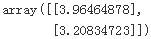

The (Mini-batch Gradient Descent's) algorithm’s progress in parameter space is less erratic不规则的 than with SGD, especially with fairly large mini-batches. As a result, Mini-batch GD will end up walking around a bit closer to the minimum than SGD. But, on the other hand, it may be harder for it to escape from local minima (in the case of problems that suffer from local minima, unlike Linear Regression as we saw earlier). Figure 4-11 shows the paths taken by the three Gradient Descent algorithms in parameter space during training. They all end up near the minimum, but Batch GD’s path actually stops at the minimum, while both Stochastic GD and Mini-batch GD continue to walk around. However, don’t forget that Batch GD takes a lot of time to take each step, and Stochastic GD and Mini-batch GD would also reach the minimum if you used a good learning schedule.
Of course, this high-degree Polynomial Regression model is severely overfitting the training data, while the linear model is underfitting it. The model that will generalize best in this case is the quadratic model. It makes sense since the data was generated using a quadratic model, but in general you won’t know what function generated the data, so how can you decide how complex your model should be? How can you tell that your model is overfitting or underfitting the data?

In (https://blog.csdn.net/Linli522362242/article/details/103587172) you used cross-validation to get an estimate of a model’s generalization performance. If a model performs well (rmse is 0.0 in DecisionTreeRegressor) on the training data but generalizes poorly according to the cross-validation metrics(rmse is 70644.94463282847 ±2939 in DecisionTreeRegressor by using cross-validation(cv=10) ), then your model is overfitting.
If it performs poorly on both, then it is underfitting. This is one way to tell when a model is too simple or too complex.
When underfitting happens it can mean that the features do not provide enough information to make good predictions, or that the model is not powerful enough. As we saw in the previous chapter, the main ways to fix underfitting are to select a more powerful model, to feed the training algorithm with better features, or to reduce the constraints on the model.
Another way is to look at the learning curves: these are plots of the model’s performance on the training set and the validation set as a function of the training set size. To generate the plots, simply train the model several times on different sized subsets of the training set. The following code defines a function that plots the learning curves of a model given some training data:
```
from sklearn.metrics import mean_squared_error
from sklearn.model_selection import train_test_split
 
def plot_learning_cures(model, X,y):
           # X_validationSet#y_validationSet
    X_train, X_val, y_train, y_val = train_test_split(X,y, test_size=0.2, random_state=10)
    train_errors, val_errors=[], [] ###MSE
    for m in range( 1, len(X_train) ):#different size of training set
        model.fit( X_train[:m], y_train[:m] )###############model
        y_train_predict = model.predict( X_train[:m] )###############model
        y_val_predict = model.predict( X_val )###############model
        train_errors.append(mean_squared_error(y_train[:m], y_train_predict))
        val_errors.append(mean_squared_error(y_val, y_val_predict))
    
    #          indices of train_errors  
    # plt.plot(list(range(len(train_errors))),np.sqrt(train_errors), "r-+", linewidth=2, label="Training set")    
    plt.plot(np.sqrt(train_errors), "r-+", linewidth=2, label="Training set")
    plt.plot(np.sqrt(val_errors), "b-", linewidth=3, label="Validation set")
    plt.legend(loc="upper right", fontsize=14)
    plt.xlabel("Training set size", fontsize=14)
    plt.ylabel("RMSE", fontsize=14)
 
lin_reg = LinearRegression()
plot_learning_cures(lin_reg, X,y)
plt.axis([0,80, 0,3])
plt.title("Figure 4-15. Learning curves")
plt.show()
```
First, let’s look at the performance on the training data: when there are just one or two instances in the training set, the model can fit them perfectly, which is why the curve starts at zero. But as new instances are added to the training set, it becomes impossible for the model to fit the training data perfectly, both because the data is noisy and because it is not linear at all. So the error on the training data goes up until it reaches a plateau(高原; 平稳时期，稳定水平; 停滞期), at which point adding new instances to the training set doesn’t make the average error much better or worse.
Now let’s look at the performance of the model on the validation data. When the model is trained on very few training instances, it is incapable of generalizing properly, which is why the validation error is initially quite big. Then as the model is shown more training examples, it learns and thus the validation error slowly goes down. However, once again a
straight line cannot do a good job modeling拟合 the data, so the error ends up at a plateau, very close to the other curve(Training set MSE).
###############################
TIP
If your model is underfitting the training data, adding more training examples will not help. You need to use a more complex
model or come up with设法拿出 better features.
###############################
Now let’s look at the learning curves of a 10th-degree polynomial model on the same data (Figure 4-16):
```
from sklearn.pipeline import Pipeline
 
polynomial_regression = Pipeline((
    ("poly_features", PolynomialFeatures(degree=10, include_bias=False)),
    ("lin_reg", LinearRegression()),
))
 
plot_learning_cures(polynomial_regression, X,y)
plt.axis([0,80,0,3])
plt.title("Figure 4-16. Learning curves for the polynomial model")
plt.show()
```
These learning curves look a bit like the previous ones, but there are two very important differences:

The error (RMSE)on the training data is much lower than with the Linear Regression model.

There is a gap(overfitting) between the curves. This means that the model performs significantly better on the training data than on the validation data, which is the hallmark显著特点 of an overfitting model. However, if you used a much larger training set, the two curves would continue to get closer.
###################
TIP
One way to improve an overfitting model is to feed it more training data until the validation error reaches the training error.
###################
THE BIAS/VARIANCE TRADEOFF
An important theoretical result of statistics and Machine Learning is the fact that a model’s generalization error can be expressed as the sum of three very different errors:

Bias偏差： This part of the generalization error is due to wrong assumptions, such as assuming that the data is linear when it is actually quadratic. A high-bias model is most likely to underfit the training data.

Variance方差： This part is due to the model’s excessive sensitivity to small variations in the training data. A model with many degrees of freedom多自由度 (such as a high-degree polynomial model) is likely to have high variance, and thus to overfit the training data.

Irreducible error不能减少的误差 : This part is due to the noisiness of the data itself. The only way to reduce this part of the error is to clean up the data (e.g., fix the data sources, such as broken sensors, or detect and remove outliers). Increasing a model’s complexity will typically increase its variance and reduce its bias. Conversely, reducing a model’s complexity increases its bias and reduces its variance. This is why it is called a tradeoff.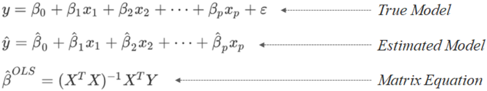
Ridge Regression (also called Tikhonov regularization) is a regularized version of Linear Regression: a regularization term equal to  is added to the cost function(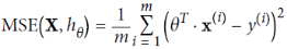). This forces the learning algorithm to not only fit the data but also keep the model weights as small as possible. Note that the regularization term should only be added to the cost function during training. Once the model is trained, you want to evaluate the model’s performance using the unregularized performance measure.
Regularization is one approach to tackle the problem of overfitting by adding additional information, and thereby shrinking the parameter values of the model to induce a penalty against complexity针对复杂性引入惩罚项.
Equation 4-8. Ridge Regression cost function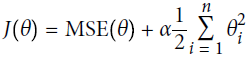
Note: is for convenient computation,  we should remove it for Practical application

Note that the bias term is not regularized (the sum starts at i = 1, not 0).


the ℓ2 norm: ,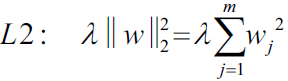
For Gradient Descent, just add 2αw or 2w to the MSE gradient vector (Equation 4-6).
+2αw (or +2α)
WARNING
It is important to scale the data (e.g., using a StandardScaler) before performing Ridge Regression, as it is sensitive to the scale of the input features. This is true of most regularized models.
```
np.random.seed(42)
m=20 #number of instances
X= 3*np.random.rand(m,1) #one feature  #X=range(0,3)
              #noise
y=1 + 0.5*X + np.random.randn(m,1)/1.5 
X_new = np.linspace(0,3, 100).reshape(100,1)
 
from sklearn.linear_model import Ridge
 
def plot_model(model_class, polynomial, alphas, **model_kargs):
    for alpha, style in zip( alphas, ("b-", "y--", "r:") ):
                ###########
        model = model_class(alpha, **model_kargs) if alpha>0 else LinearRegression()
        if polynomial:
            model = Pipeline([
                ("poly_features", PolynomialFeatures(degree=10, include_bias=False)),
                ("std_scaler", StandardScaler()),
                ("regul_reg", model) #regulized regression
            ])
        model.fit(X,y)
        y_new_regul = model.predict(X_new)
        lw = 5 if alpha>0 else 1
        plt.plot(X_new, y_new_regul, style, linewidth=lw, label=r"$\alpha = {}$".format(alpha) )
    plt.plot(X,y, "b.", linewidth=3)
    plt.legend(loc="upper left", fontsize=15)
    plt.xlabel("$x_1$", fontsize=18)
    plt.axis([0,3, 0,4])
 
plt.figure(figsize=(8,4) )
plt.subplot(121)
           ######
plot_model(Ridge, polynomial=False, alphas=(0,10,100), random_state=42)#plain Ridge models are used, leading to 
plt.ylabel("$y$", rotation=0, fontsize=18)
 
plt.subplot(122)
           ######
plot_model(Ridge, polynomial=True, alphas=(0,10**-5, 1), random_state=42)
plt.title("Figure 4-17. Ridge Regression")
plt.show()
```
If α = 0 then Ridge Regression is just Linear Regression.
If α is very large, then all weights end up very close to zero and the result is a flat line going through the data’s mean.
Figure 4-17 shows several Ridge models trained on some linear data using different α value. On the left, plain Ridge models are used, leading to linear predictions. On the right, the data is first expanded using PolynomialFeatures(degree=10), then it is scaled using a StandardScaler, and finally the Ridge models are applied to the resulting features: this is Polynomial Regression with Ridge regularization. Note how increasing α leads to flatter (i.e., less extreme, more reasonable) predictions; this reduces the model’s variance but increases its bias.(Regularization is one approach to tackle the problem of overfitting by adding additional information, and thereby shrinking the parameter values of the model to induce a penalty against complexity针对复杂性引入惩罚项.)

As with Linear Regression, we can perform Ridge Regression either by computing a closed-form equation or by performing Gradient Descent. The pros and cons are the same. Equation 4-9 shows the closed-form solution (where A is the n × n identity单位 matrix A( A square matrix full of 0s except for 1s on the main diagonal (top-left to bottom-right). ) except with a 0 in the top-left cell, corresponding to the bias term ).

Equation 4-9. Ridge Regression closed-form solution

Note: Normal Equation(a closed-form equation)
ridge_reg = Ridge(alpha=1, solver="cholesky", random_state=42)
ridge_reg.fit(X,y)
ridge_reg.predict([[1.5]])
ridge_reg = Ridge(alpha=1, solver="sag", random_state=42)
ridge_reg.fit(X,y)
ridge_reg.predict([[1.5]])
sgd_reg = SGDRegressor( penalty="l2", max_iter=1000, tol=1e-3, random_state=42)
sgd_reg.fit(X,y.ravel()) #X= 3*np.random.rand(m,1) #y=1 + 0.5*X + np.random.randn(m,1)/1.5
sgd_reg.predict([[1.5]])
The penalty hyperparameter sets the type of regularization term to use. Specifying "l2" indicates that you want SGD to add a regularization term to the cost function equal to half the square of the ℓ2 norm of the weight vector: this is simply Ridge Regression.
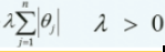
Least Absolute Shrinkage and Selection Operator Regression (simply called Lasso Regression) is another regularized version of Linear Regression: just like Ridge Regression, it adds a regularization term to the cost function, but it uses the ℓ1 norm of the weight vector instead of half the square of the ℓ2 norm
Equation 4-10. Lasso Regression cost function
OR
The Lasso cost function is not differentiable无法进行微分运算 at θi = 0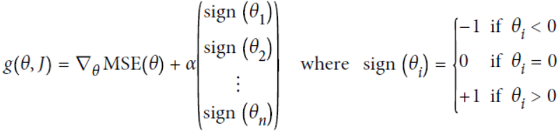
Note: here ==
Figure 4-18 shows the same thing as Figure 4-17 but replaces Ridge models with Lasso models and uses smaller α values.
```
from sklearn.linear_model import Lasso
 
plt.figure(figsize=(8,4))
plt.subplot(121)
plot_model(Lasso, polynomial=False, alphas=(0, 0.1, 1), random_state=42)
plt.ylabel("$y$", rotation=0, fontsize=18)
 
plt.subplot(122)
plot_model(Lasso, polynomial=True, alphas=(0, 10**-7, 1), random_state=42)
plt.title("Figure 4-18. Lasso Regression")
plt.show()
```
An important characteristic of Lasso Regression is that it tends to completely eliminate the weights of the least important features最不重要 (i.e., set them to zero). For example, the dashed line in the right plot on Figure 4-18 (with α = 10-7) looks quadratic, almost linear(compared to Figure 4-17 ):since all the weights for the high-degree polynomial features are equal to zero. In other words, Lasso Regression automatically performs feature selection and outputs a sparse model (i.e., with few nonzero feature weights).

Elastic Net is a middle ground between Ridge Regression and Lasso Regression. The regularization term is a simple mix of both Ridge and Lasso’s regularization terms, and you can control the mix ratio r. When r = 0, Elastic Net is equivalent to Ridge Regression, and when r = 1, it is equivalent to Lasso Regression (see Equation 4-12).
Equation 4-12. Elastic Net cost function

from sklearn.linear_model import ElasticNet
elastic_net = ElasticNet(alpha=0.1, l1_ratio=0.5, random_state=42)
elastic_net.fit(X,y)
elastic_net.predict([[1.5]])#elastic_net.intercept_, elastic_net.coef_ # (array([1.08639303]), array([0.30462619]))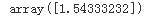

https://blog.csdn.net/Linli522362242/article/details/104070847

t1a, t1b, t2a, t2b = -1, 3, -1.5, 1.5
 
# ignoring bias term
theta1s = np.linspace(t1a, t1b, 500) # 500 points
theta2s = np.linspace(t2a, t2b, 500) # 500 points
theta1, theta2 = np.meshgrid(theta1s, theta2s)
                            #theta1: 500pts*500 500 points are copied along the points on coordinate axis theta2 
                            #theta2: 500pts*500 500 points are copied along the points on coordinate axis theta1
theta = np.c_[theta1.ravel(), theta2.ravel()] #(250000, 250000) #corresponding to (features1, feature2)
Xr = np.array([
                [-1,    1], #[feature1, feature2]
                [-0.3, -1], #[feature1, feature2]
                [1,   0.1]  #[feature1, feature2]
              ])
#Xt.T
#feature1, ..., feature1
#feature2, ..., feature2
#...
#yi = 2 * Xi1 + 0.5 * Xi2
yr = 2*Xr[:, :1] + 0.5*Xr[:, 1:] #instances' labels are stored in multiple rows & one column
#yr.T
#array([
#       [label1, label2,...]
#     ])
 
#MSE            #hiding: shape(250000, 3)-shape(1, 3)*250000
J = ( 1/len(Xr) *np.sum(( theta.dot(Xr.T) -yr.T )**2, axis=1 )).reshape(theta1.shape) # MSE at (500,500)
 
N1 = np.linalg.norm(theta, ord=1, axis=1).reshape(theta1.shape)#L1 norm: row_i = sum(|theta_i1| + |theta_i2|) 
N2 = np.linalg.norm(theta, ord=2, axis=1).reshape(theta1.shape)#L2 norm: row_i=sqrt(sum(theta_i1 **2 + theta_i2 **2) )
 
                # np.argmin(J): minimum value's index==166874 after the J being flatten
theta_min_idx = np.unravel_index( np.argmin(J), J.shape) #get the index==(333, 374) in orginal J (without being flatten)
theta1_min, theta2_min=theta1[theta_min_idx],theta2[theta_min_idx] #get the corresponding minimum thata values
#theta1_min, theta2_min #(1.9979959919839678, 0.5020040080160322)
 
t_init = np.array([[0.25], #theta1
                   [-1]    #theta2
                  ]) #start point


                          #L1 norm, L2 norm    
def bgd_path(theta, X, y, l1_alpha, l2_alpha, core=1, eta=0.1, n_iterations=50):
    path = [theta]
    for iteration in range(n_iterations):
        #formula gradients = 2/m * X_b.T.dot( X_b.dot(theta)-y )                    # 2*
        gradients = core* 2/len(X) * X.T.dot( X.dot(theta)-y ) + l1_alpha*np.sign(theta) + 2*l2_alpha*theta
        theta = theta -eta*gradients                            # l1: alpha                #l2: alpha
        path.append(theta)
    return np.array(path)

plt.figure( figsize=(12,8) )
               #initial theta=0 in Lasso, initial theta=1 in Ridge 
for i, N, l1_alpha, l2_alpha, title in ( (0, N1, 0.5, 0, "Lasso"), (1, N2, 0, 0.1, "Ridge") ):
    #J:unregularized MSE cost function;  JR:regularized MSE cost function
    JR = J + l1_alpha*N1 + l2_alpha* N2**2  #cost function
    
    #get current minimum of theta1 and theta2 in regularized MSE cost function
    thetaR_min_idx = np.unravel_index(np.argmin(JR), JR.shape)
    theta1R_min, theta2R_min = theta1[thetaR_min_idx], theta2[thetaR_min_idx]
    
    #contour levels
    #min-max scaling    x_new=x-min/(max-min) ==> x=x_new*(max-min)+min
    levelsJ = (np.exp(np.linspace(0,1,20)) -1) *( np.max(J)-np.min(J) ) + np.min(J)
    levelsJR =(np.exp(np.linspace(0,1,20)) -1) *( np.max(JR)-np.min(JR) ) + np.min(JR)
    levelsN = np.linspace(0, np.max(N), 10)
    
    path_J= bgd_path(t_init, Xr, yr, l1_alpha=0, l2_alpha=0) #an unregularized MSE cost function(α = 0)
    path_JR = bgd_path(t_init, Xr, yr, l1_alpha, l2_alpha) #a regularized MSE cost function
    path_N = bgd_path(t_init, Xr, yr, np.sign(l1_alpha)/3, np.sign(l2_alpha), core=0)
    
    plt.subplot(221 + i*2)
    plt.grid(True)
    plt.axhline(y=0, color='k')
    plt.axvline(x=0, color='k')
    #J:unregularized MSE cost function
    #the background contours (ellipses) represent an unregularized MSE cost function(α = 0)
    plt.contourf(theta1, theta2, J, levels=levelsJ, alpha=0.9)
    #The foreground contours (diamonds) represent the ℓ1 penalty
    plt.contour(theta1, theta2, N, levels=levelsN)
    
    plt.plot(path_J[:,0], path_J[:,1], "w-o")#the white circles show the Batch Gradient Descent path that cost function
    plt.plot(path_N[:,0], path_N[:,1], "y-^")#the triangles show the BGD path for this penalty only (α → ∞).
    plt.plot(theta1_min, theta2_min, "bs") #minimum values of theta1 , theta2
    plt.title(r"$\ell_{}$ penalty".format(i+1), fontsize=16)
    plt.axis([t1a,t1b, t2a,t2b])
    if i==1:
        plt.xlabel(r"$\theta_1$", fontsize=20)
    plt.ylabel(r"$\theta_2$", fontsize=20, rotation=0)
    
    plt.subplot(222 + i*2)
    plt.grid(True)
    plt.axhline(y=0, color="k")
    plt.axvline(x=0, color="k")
    #JR:regularized MSE cost function
    plt.contourf(theta1, theta2, JR, levels=levelsJR, alpha=0.9)
               
    plt.plot(path_JR[:,0], path_JR[:,1], "w-o")#the white circles show the Batch Gradient Descent path that cost func
    plt.plot(theta1R_min, theta2R_min, "bs") #minimum values of theta1 , theta2
    plt.title(title, fontsize=16)
    plt.axis([t1a,t1b, t2a,t2b]) 
    if i ==1:
        plt.xlabel(r"$\theta_1$", fontsize=20)
    
plt.show()

You can get a sense of why this is the case by looking at above Figure: on the top-left plot, the background contours (ellipses) represent an unregularized MSE cost function (α = 0), and the white circles show the Batch Gradient Descent path with that cost function. The foreground contours (diamonds) represent the ℓ1 penalty, and the yellow triangles show the BGD path for this penalty only (α → ∞). Notice how the path first reaches θ1 = 0, then rolls down a gutter until it reaches θ2 = 0.

On the top-right plot, the contours represent the same cost function plus an ℓ1 penalty with α = 0.5. The global minimum is on the θ2 = 0 axis. BGD first reaches θ2 = 0( Lasso Regression automatically performs feature selection and outputs a sparse model (i.e., with few nonzero feature weights) ), then rolls down the gutter until it reaches the global minimum.

The two bottom plots show the same thing but uses an ℓ2 penalty(with α = 0.1) instead. The regularized minimum is closer to θ = 0 than the unregularized minimum , but(On Ridge) the weights do not get fully eliminated 但权重不能完全消除.
################################
TIP
On the Lasso cost function, the BGD path tends to bounce反弹 across the gutter toward the end. This is because the slope changes abruptly at θ2 = 0( Lasso Regression automatically performs feature selection and outputs a sparse model (i.e., with few nonzero feature weights) ). You need to gradually reduce the learning rate in order to actually converge to the global minimum.

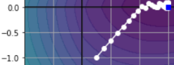
A very different way to regularize iterative learning algorithms such as Gradient Descent is to stop training as soon as the validation error reaches a minimum. This is called early stopping. Figure 4-20 shows a complex model (in this case a high-degree Polynomial Regression model) being trained using Batch Gradient Descent. As the epochs go by, the algorithm learns and its prediction error (RMSE) on the training set naturally goes down, and so does its prediction error on the validation set. However, after a while the validation error stops decreasing and actually starts to go back up. This indicates that the model has started to overfit the training data. With early stopping you just stop training as soon as the validation error reaches the minimum. It is such a simple and efficient regularization technique that Geoffrey Hinton called it a “beautiful free lunch.”

np.random.seed(42)
m=100
X = 6*np.random.rand(m,1)-3
y = 2+X + 0.5 * X**2 + np.random.randn(m,1)
X_train, X_val, y_train, y_val = train_test_split(X[:50], y[:50].ravel(), test_size=0.5, random_state=10)
 
poly_scaler = Pipeline([
    ("poly_features", PolynomialFeatures(degree=90, include_bias=False)),
    ("std_scaler", StandardScaler())
])
 
X_train_poly_scaled = poly_scaler.fit_transform(X_train)
#use the mean and variance which is from StandardScaler() of poly_scaler.fit_transform(X_train)
X_val_poly_scaled = poly_scaler.transform(X_val)
 
#Note that with warm_start=True, when the fit() method is called, it just continues
#training where it left off instead of restarting from scratch.
sgd_reg = SGDRegressor(max_iter=1, tol=-np.infty,warm_start=True,
                      penalty=None, learning_rate="constant", eta0=0.0005, random_state=42)
n_epochs=500
train_errors, val_errors=[],[]
for epoch in range(n_epochs):
    sgd_reg.fit(X_train_poly_scaled, y_train)
    y_train_predict = sgd_reg.predict(X_train_poly_scaled)
    y_val_predict = sgd_reg.predict(X_val_poly_scaled)
    train_errors.append(mean_squared_error(y_train, y_train_predict))
    val_errors.append(mean_squared_error(y_val, y_val_predict))
    
best_epoch = np.argmin(val_errors)
best_val_rmse = np.sqrt(val_errors[best_epoch])
 
plt.annotate("Best model",
             xy=(best_epoch, best_val_rmse),
             xytext = (best_epoch, best_val_rmse+1),
             ha="center",
             arrowprops=dict(facecolor="black", shrink=0.05),
             fontsize=16,
            )
 
best_val_rmse -= 0.03 # just to make the graph look better (move the horizontal blackline down -0.03)
plt.plot([0, n_epochs], [best_val_rmse, best_val_rmse], "k:", linewidth=2) # horizontal black line
        #hiding: list(range(0, n_epochs,1)),
plt.plot( np.sqrt(val_errors), "b-", linewidth=3, label="Validation set")
plt.plot( np.sqrt(train_errors), "r--", linewidth=2, label="Training set")
plt.legend(loc="upper right", fontsize=14)
plt.xlabel("Epoch", fontsize=14)
plt.ylabel("RMSE", fontsize=14)
plt.title("Figure 4-20. Early stopping regularization")
plt.show()

#################################
TIP
With Stochastic and Mini-batch Gradient Descent, the curves are not so smooth, and it may be hard to know whether you have reached the minimum or not. One solution is to stop only after the validation error has been above the minimum for some time (when you are confident that the model will not do any better), then roll back the model parameters to the point where the validation error was at a minimum.
#################################

Here is a basic implementation of early stopping:

from sklearn.base import clone
 
poly_scaler = Pipeline([
    ("poly_features", PolynomialFeatures(degree=90, include_bias=False)),
    ("std_scaler", StandardScaler())
])
 
X_train_poly_scaled = poly_scaler.fit_transform(X_train)
#use the mean and variance which is from StandardScaler() of poly_scaler.fit_transform(X_train)
X_val_poly_scaled = poly_scaler.transform(X_val)
 
#Note that with warm_start=True, when the fit() method is called, it just continues training where it left
#off instead of restarting from scratch.
sgd_reg = SGDRegressor(max_iter=1, tol=-np.infty, warm_start=True,
                      penalty=None, learning_rate="constant", eta0=0.0005, random_state=42)
 
minimum_val_error = float("inf")
best_epoch = None
best_model = None
for epoch in range(1000):
    sgd_reg.fit(X_train_poly_scaled, y_train)
    y_val_predict = sgd_reg.predict(X_val_poly_scaled)##################
    val_error = mean_squared_error(y_val, y_val_predict)
    if val_error < minimum_val_error:
        minimum_val_error = val_error
        best_epoch = epoch
        best_model = clone(sgd_reg)

best_epoch, best_model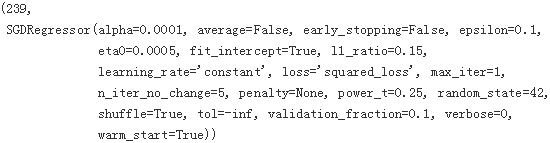

some regression algorithms can be used for classification as well (and vice versa). Logistic Regression (also called Logit Regression) is commonly used to estimate the probability that an instance belongs to a particular class (e.g., what is the probability that this email is spam?). If the estimated probability is greater than 50%, then the model predicts that the instance belongs to that class (called the positive class, labeled “1”), or else it predicts that it does not (i.e., it belongs to the negative class, labeled “0”). This makes it a binary classifier.

a Logistic Regression model computes a weighted sum of the input fea
tures (plus a bias term), but instead of outputting the result directly like the Linear Regression model does, it outputs the logistic of this result (see Equation 4-13).

Equation 4-13. Logistic Regression model estimated probability (vectorized form)

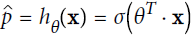
The logistic—also called the logit, noted σ(·)—is a sigmoid function (i.e., S-shaped) that outputs a number between 0 and 1. It is defined as shown in Equation 4-14 and Figure 4-21.

Equation 4-14. Logistic function

Once the Logistic Regression model has estimated the probability that an instance x belongs to the positive class, it can make its prediction ŷ easily (see Equation 4-15).

Equation 4-15. Logistic Regression model prediction

Notice that σ(t) < 0.5 when t < 0, and σ(t) ≥ 0.5 when t ≥ 0, so a Logistic Regression model predicts 1 if t==  is positive(>=0.5), and 0 if it is negative(<0.5).

Note:   and t= and  and
The objective of training is to set the parameter vector θ so that the model estimates high probabilities for positive instances (y =1) and low probabilities for negative instances (y = 0). This idea is captured by the cost function shown in Equation 4-16 for a single training instance x.
Equation 4-16. Cost function of a single training instance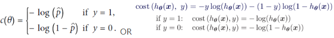
This cost function makes sense because –log(t) grows very large when t approaches 0 (e.g. -log(0.1)==1,
-log(0.0000000001)==10,

so the cost will be large if the model estimates a probability close to 0 for a positive instance(if y=1, >=0.5, >0), the cost will be close to 0 if the estimated probability is close to 1 for a positive instance(if y=1, >=0.5, , >0).
and the cost will also be very large if the model estimates a probability close to 1 for a negative instance(if y=0, <0.5, , <0). and the cost will be close to 0 if the estimated probability is close to 0 for a negative instance(if y=0, <0.5, , <0) ;
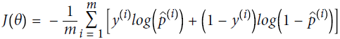
Equation 4-17. Logistic Regression cost function (log loss)
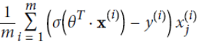
Equation 4-18. Logistic cost function partial derivatives(The bad news is that there is no known closed-form equation to compute the value of θ that minimizes this cost function (there is no equivalent of the Normal Equation). But the good news is that this cost function is convex, so Gradient Descent (or any other optimization algorithm) is guaranteed to find the global minimum(, the ==; Once the left theta(next step) == right theta, we at get the minimum of cost function)
This equation(Equation 4-18) looks very much like Equation 4-5: for each instance it computes the prediction error and multiplies it by the jth feature value, and then it computes the average over all training instances. Once you have the gradient vector containing all the partial derivatives you can use it in the Batch Gradient Descent algorithm. That’s it: you now know how to train a Logistic Regression model. For Stochastic GD you would of course just take one instance at a time, and for Mini-batch GD you would use a mini-batch at a time.

Equation 4-6. Gradient vector of the cost function ()
Note: X's columns in each row(each instance) are features [x0==1, x1, x2, ..., xn], [theta is theta_0, theta_1, .., theta_n]; Note Xij, i is row index, j is column index(feature/weight index)
cost function ==> Partial derivatives of the cost fucntion==>gradient vector of the cost function
################################################################

Decision Boundaries

Let’s use the iris dataset to illustrate Logistic Regression. This is a famous dataset that contains the sepal萼片 and petal 花瓣 length and width of 150 iris flowers of three different species: Iris-Setosa, Iris-Versicolor, and Iris-Virginica (see Figure 4-22).

Let’s try to build a classifier to detect the Iris-Virginica type based only on the petal width feature. First let’s load the data:

from sklearn import datasets
iris = datasets.load_iris()
type(iris)

for k,v in iris.items():
    print(k,v)

...

list(iris.keys())

X = iris["data"][:,3:] #petal width
y = (iris["target"]==2).astype(np.int) ## 1 if Iris-Virginica, else 0

Now let’s train a Logistic Regression model:
Note: To be future-proof we set solver="lbfgs" since this will be the default value in Scikit-Learn 0.22.

from sklearn.linear_model import LogisticRegression

log_reg = LogisticRegression(solver="lbfgs", random_state=42)
log_reg.fit(X,y)

Let’s look at the model’s estimated probabilities for flowers with petal widths varying from 0 to 3 cm (Figure 4-23):

X_new = np.linspace(0,3, 1000).reshape(-1,1) #1000rows, 1 column
y_proba = log_reg.predict_proba(X_new)
y_proba

decision_boundary = X_new[y_proba[:, 1]>=0.5][0] #the probability of Iris-Virginica flowers >=0.5 

plt.figure(figsize=(8,3))
plt.plot(X[y==0], y[y==0], "bs") # Not Iris-Virginica flowers (represented by squares)
plt.plot(X[y==1], y[y==1], "g^") # Iris-Virginica flowers (represented by triangles)
plt.plot([decision_boundary, decision_boundary], [0,1], "k:", linewidth=2)
plt.plot(X_new, y_proba[:,1], "g-", linewidth=2, label="Iris-Virginica")
plt.plot(X_new, y_proba[:,0], "b--", linewidth=2, label="Not Iris-Virginica")

plt.text(decision_boundary+0.02, 0.15, "Decision boundary", fontsize=14, color="k", ha="center")
plt.arrow(decision_boundary, 0.08, -0.3, 0, head_width=0.05, head_length=0.1, fc="b", ec="k") #-->
plt.arrow(decision_boundary, 0.92, 0.3, 0, head_width=0.05, head_length=0.1, fc="g", ec="k")  #<--
plt.xlabel("Petal width (cm)", fontsize=14)
plt.ylabel("Probability", fontsize=14)
plt.legend(loc="center left", fontsize=14)
plt.axis([0,3, -0.02,1.02])
plt.show()

The petal width of Iris-Virginica flowers (represented by triangles) ranges from 1.4 cm to 2.5 cm, while the other iris flowers (represented by squares) generally have a smaller petal width, ranging from 0.1 cm to 1.8 cm. Notice that there is a bit of overlap.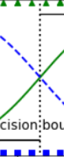

Above about 2 cm the classifier is highly confident that the flower is an Iris-Virginica (it outputs a high probability to that class), while below 1 cm it is highly confident that it is not an Iris-Virginica (high probability for the “Not Iris-Virginica” class). In between these extremes, the classifier is unsure. However, if you ask it to predict the class (using the predict() method rather than the predict_proba() method), it will return whichever class is the most likely. Therefore, there is a decision boundary at around 1.6 cm where both probabilities are equal to 50%: if the petal width is higher than 1.6 cm, the classifier will predict that the flower is an Iris-Virginica, or else it will predict that it is not (even if it is not very confident):

decision_boundary

log_reg.predict([[1.7], [1.5]])

# 1: Iris-Virginica, 0: not an Iris-Virginica

Figure 4-24 shows the same dataset but this time displaying two features: petal width and length. Once trained, the Logistic Regression classifier can estimate the probability that a new flower is an Iris-Virginica based on these two features. The dashed line represents the points where the model estimates a 50% probability: this is the model’s decision boundary. Note that it is a linear boundary. Each parallel line represents the points where the model outputs a specific probability, from 15% (bottom left) to 90% (top right). All the flowers beyond the top-right line have an over 90% chance of being Iris-Virginica according to the model.

from sklearn.linear_model import LogisticRegression

X = iris["data"][:, (2,3)] #petal length, petal width
y = (iris["target"]==2).astype(np.int) # 1 if Iris-Virginica, else 0
                                            #The higher the value of C, the less the model is regularized.
log_reg = LogisticRegression(solver="lbfgs", C=10**10, random_state=42) #C is alpha's inverse
log_reg.fit(X,y)

Note: and = and OR

= =,
==1 , is the intercept of decision boundary line(called best fit line)

an input of 0 (t=0.0)was our center line to split things classified as a 1(positive class) and a 0(negative class), so
are best fit line or decision boundary line; x1 is Petal length, x2 is Petal width

x0, x1 =np.meshgrid(
    np.linspace(2.9, 7,  500).reshape(-1,1),#[[500 rows] 1 column]
    np.linspace(0.8, 2.7,200).reshape(-1,1),#[[200 rows] 1 column]
)
#x0: [[2.9,...500 columns...,7]...200 rows...[2.9,...500...,7]]
#x1: [[0.8,...500 columns...,0.8]...200 rows...[2.7,...500...,2.7]]

X_new = np.c_[x0.ravel(), x1.ravel()] #[200*500, 200*500]
y_proba = log_reg.predict_proba(X_new)

plt.figure(figsize=(10,4))
plt.plot(X[y==0, 0], X[y==0, 1], "bs")#Petal length, Petal width of not iris-Virginca
plt.plot(X[y==1, 0], X[y==1, 1], "y^")#Petal length, Petal width of iris-Virginca

#from matplotlib.colors import ListedColormap
#colors=("blue", "red","green")
#cmap=ListedColormap(colors)
zz = y_proba[:,1].reshape(x0.shape) #(200,500)
contour=plt.contour(x0, x1, zz, cmap=plt.cm.brg) #plt.cm.brg==cmap=blue-red-green

left_right = np.array([2.9, 7])
            #theta_1 correspondings to Petal length                     #theta_2 correspondings to Pental width   
boundary = -(log_reg.coef_[0][0]*left_right + log_reg.intercept_[0] ) / log_reg.coef_[0][1]
plt.plot(left_right, boundary, "k--", linewidth=3)#decision boundary

plt.clabel(contour, inline=True, fontsize=12)
plt.text(3.5, 1.5, "Not Iris virginica", fontsize=14, color="b", ha="center")
plt.text(6.5, 2.3, "Iris virginica", fontsize=14, color="g", ha="center")
plt.axis([2.9,7, 0.8,2.7])
plt.xlabel("Petal length", fontsize=14)
plt.ylabel("Petal width", fontsize=14)
plt.show()

Just like the other linear models, Logistic Regression models can be regularized using ℓ1 or ℓ2 penalties. Here, Scitkit-Learn actually adds an ℓ2 penalty by default since solver="lbfgs" .

The hyperparameter controlling the regularization strength of a Scikit-Learn LogisticRegression model is not alpha (as in other linear models), but its inverse: C. The higher the value of C, the less the model is regularized.

######################################################extra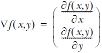

this gradient means that we’ll move in the x direction by amount and in the y direction by amount. The function f(x,y) needs to be defined and differentiable around the points where it’s being evaluated.
The magnitude, or step size, we’ll take is given by the parameter . In vector notation we can write the gradient ascent algorithm as This step is repeated until we reach a stopping condition: either a specified number of
steps or the algorithm is within a certain tolerance margin.

Softmax Regression

LIQING LIN

发布了58 篇原创文章 · 获赞 40 · 访问量 1万+

私信关注

Decision Boundaries

Softmax Regression

猜你喜欢