第一部分:线性回归
主要内容包括:
- 线性回归的基本要素
- 线性回归模型从零开始的实现
- 线性回归模型使用pytorch的简洁实现
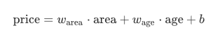
模型:
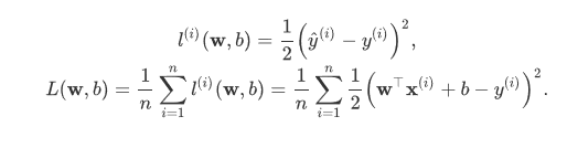
损失函数:
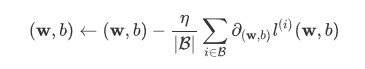
优化函数 - 随机梯度下降:
小批量随机梯度下降(mini-batch stochastic gradient descent)在深度学习中被广泛使用。它的算法很简单:先选取一组模型参数的初始值,如随机选取;接下来对参数进行多次迭代,使每次迭代都可能降低损失函数的值。在每次迭代中,先随机均匀采样一个由固定数目训练数据样本所组成的小批量(mini-batch)B,然后求小批量中数据样本的平均损失有关模型参数的导数(梯度),最后用此结果与预先设定的一个正数的乘积作为模型参数在本次迭代的减小量。
矢量计算:
在模型训练或预测时,我们常常会同时处理多个数据样本并用到矢量计算。在介绍线性回归的矢量计算表达式之前,让我们先考虑对两个向量相加的两种方法。
向量相加的一种方法是,将这两个向量按元素逐一做标量加法。
向量相加的另一种方法是,将这两个向量直接做矢量加法。
import torch
import time

# init variable a, b as 1000 dimension vector
n = 1000
a = torch.ones(n)
b = torch.ones(n)
# define a timer class to record time
class Timer(object):
    """Record multiple running times."""
    def __init__(self):
        self.times = []
        self.start()

    def start(self):
        # start the timer
        self.start_time = time.time()

    def stop(self):
        # stop the timer and record time into a list
        self.times.append(time.time() - self.start_time)
        return self.times[-1]

    def avg(self):
        # calculate the average and return
        return sum(self.times)/len(self.times)

    def sum(self):
        # return the sum of recorded time
        return sum(self.times)
现在我们可以来测试了。首先将两个向量使用for循环按元素逐一做标量加法。
timer = Timer()
c = torch.zeros(n)
for i in range(n):
    c[i] = a[i] + b[i]
'%.5f sec' % timer.stop()
另外是使用torch来将两个向量直接做矢量加法:
timer.start()
d = a + b
'%.5f sec' % timer.stop()
线性回归模型从零开始的实现
# import packages and modules
%matplotlib inline
import torch
from IPython import display
from matplotlib import pyplot as plt
import numpy as np
import random

print(torch.__version__)
生成数据集
# set input feature number
num_inputs = 2
# set example number
num_examples = 1000

# set true weight and bias in order to generate corresponded label
true_w = [2, -3.4]
true_b = 4.2

features = torch.randn(num_examples, num_inputs,
                      dtype=torch.float32)
labels = true_w[0] * features[:, 0] + true_w[1] * features[:, 1] + true_b
labels += torch.tensor(np.random.normal(0, 0.01, size=labels.size()),
                       dtype=torch.float32)
使用图像来展示生成的数据
plt.scatter(features[:, 1].numpy(), labels.numpy(), 1);
读取数据集
def data_iter(batch_size, features, labels):
    num_examples = len(features)
    indices = list(range(num_examples))
    random.shuffle(indices)  # random read 10 samples
    for i in range(0, num_examples, batch_size):
        j = torch.LongTensor(indices[i: min(i + batch_size, num_examples)]) # the last time may be not enough for a whole batch
        yield  features.index_select(0, j), labels.index_select(0, j)
batch_size = 10

for X, y in data_iter(batch_size, features, labels):
    print(X, '\n', y)
    break
初始化模型参数
w = torch.tensor(np.random.normal(0, 0.01, (num_inputs, 1)), dtype=torch.float32)
b = torch.zeros(1, dtype=torch.float32)

w.requires_grad_(requires_grad=True)
b.requires_grad_(requires_grad=True)
定义模型
def linreg(X, w, b):
    return torch.mm(X, w) + b
定义损失函数
使用的是均方误差损失函数:
def squared_loss(y_hat, y):
    return (y_hat - y.view(y_hat.size())) ** 2 / 2
定义优化函数
优化函数使用的是小批量随机梯度下降:
def sgd(params, lr, batch_size):
    for param in params:
        param.data -= lr * param.grad / batch_size # ues .data to operate param without gradient track
训练
# super parameters init
lr = 0.03
num_epochs = 5

net = linreg
loss = squared_loss

# training
for epoch in range(num_epochs):  # training repeats num_epochs times
    # in each epoch, all the samples in dataset will be used once

    # X is the feature and y is the label of a batch sample
    for X, y in data_iter(batch_size, features, labels):
        l = loss(net(X, w, b), y).sum()
        # calculate the gradient of batch sample loss
        l.backward()
        # using small batch random gradient descent to iter model parameters
        sgd([w, b], lr, batch_size)
        # reset parameter gradient
        w.grad.data.zero_()
        b.grad.data.zero_()
    train_l = loss(net(features, w, b), labels)
    print('epoch %d, loss %f' % (epoch + 1, train_l.mean().item()))
线性回归模型使用pytorch的简洁实现
import torch
from torch import nn
import numpy as np
torch.manual_seed(1)

print(torch.__version__)
torch.set_default_tensor_type('torch.FloatTensor')
num_inputs = 2
num_examples = 1000

true_w = [2, -3.4]
true_b = 4.2

features = torch.tensor(np.random.normal(0, 1, (num_examples, num_inputs)), dtype=torch.float)
labels = true_w[0] * features[:, 0] + true_w[1] * features[:, 1] + true_b
labels += torch.tensor(np.random.normal(0, 0.01, size=labels.size()), dtype=torch.float)
import torch.utils.data as Data

batch_size = 10

# combine featues and labels of dataset
dataset = Data.TensorDataset(features, labels)

# put dataset into DataLoader
data_iter = Data.DataLoader(
    dataset=dataset,            # torch TensorDataset format
    batch_size=batch_size,      # mini batch size
    shuffle=True,               # whether shuffle the data or not
    num_workers=2,              # read data in multithreading
)
for X, y in data_iter:
    print(X, '\n', y)
    break
class LinearNet(nn.Module):
    def __init__(self, n_feature):
        super(LinearNet, self).__init__()      # call father function to init
        self.linear = nn.Linear(n_feature, 1)  # function prototype: `torch.nn.Linear(in_features, out_features, bias=True)`

    def forward(self, x):
        y = self.linear(x)
        return y

net = LinearNet(num_inputs)
print(net)
# ways to init a multilayer network
# method one
net = nn.Sequential(
    nn.Linear(num_inputs, 1)
    # other layers can be added here
    )

# method two
net = nn.Sequential()
net.add_module('linear', nn.Linear(num_inputs, 1))
# net.add_module ......

# method three
from collections import OrderedDict
net = nn.Sequential(OrderedDict([
          ('linear', nn.Linear(num_inputs, 1))
          # ......
        ]))

print(net)
print(net[0])
from torch.nn import init

init.normal_(net[0].weight, mean=0.0, std=0.01)
init.constant_(net[0].bias, val=0.0)  # or you can use `net[0].bias.data.fill_(0)` to modify it directly
for param in net.parameters():
    print(param)
loss = nn.MSELoss()    # nn built-in squared loss function
                       # function prototype: `torch.nn.MSELoss(size_average=None, reduce=None, reduction='mean')`
import torch.optim as optim

optimizer = optim.SGD(net.parameters(), lr=0.03)   # built-in random gradient descent function
print(optimizer)  # function prototype: `torch.optim.SGD(params, lr=, momentum=0, dampening=0, weight_decay=0, nesterov=False)`
num_epochs = 3
for epoch in range(1, num_epochs + 1):
    for X, y in data_iter:
        output = net(X)
        l = loss(output, y.view(-1, 1))
        optimizer.zero_grad() # reset gradient, equal to net.zero_grad()
        l.backward()
        optimizer.step()
    print('epoch %d, loss: %f' % (epoch, l.item()))
# result comparision
dense = net[0]
print(true_w, dense.weight.data)
print(true_b, dense.bias.data)
第二部分:softmax和分类模型
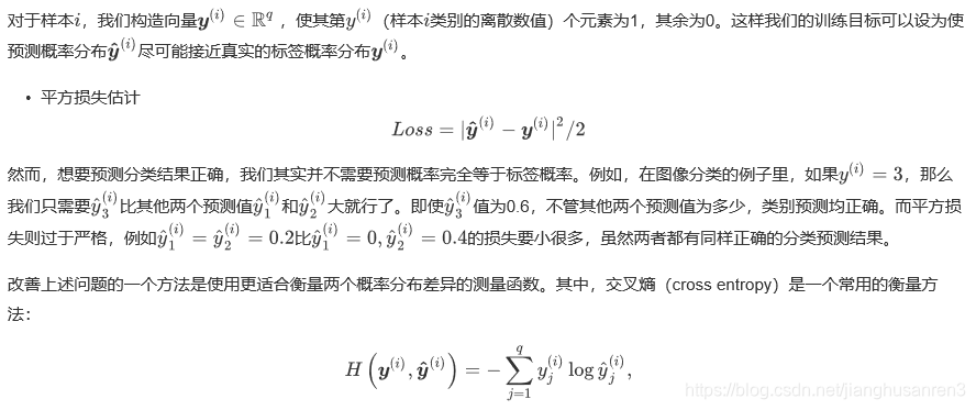
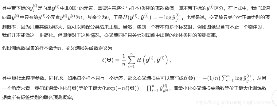
交叉熵损失函数
获取Fashion-MNIST训练集和读取数据
# import needed package
%matplotlib inline
from IPython import display
import matplotlib.pyplot as plt

import torch
import torchvision
import torchvision.transforms as transforms
import time

import sys
sys.path.append("/home/kesci/input")
import d2lzh1981 as d2l

print(torch.__version__)
print(torchvision.__version__)
mnist_train = torchvision.datasets.FashionMNIST(root='/home/kesci/input/FashionMNIST2065', train=True, download=True, transform=transforms.ToTensor())
mnist_test = torchvision.datasets.FashionMNIST(root='/home/kesci/input/FashionMNIST2065', train=False, download=True, transform=transforms.ToTensor())
class torchvision.datasets.FashionMNIST(root, train=True, transform=None, target_transform=None, download=False)
- root(string)– 数据集的根目录,其中存放processed/training.pt和processed/test.pt文件。
- train(bool, 可选)– 如果设置为True,从training.pt创建数据集,否则从test.pt创建。
- download(bool, 可选)– 如果设置为True,从互联网下载数据并放到root文件夹下。如果root目录下已经存在数据,不会再次下载。
- transform(可被调用 , 可选)– 一种函数或变换,输入PIL图片,返回变换之后的数据。如:transforms.RandomCrop。
target_transform(可被调用 , 可选)– 一种函数或变换,输入目标,进行变换。
# show result
print(type(mnist_train))
print(len(mnist_train), len(mnist_test))
# 我们可以通过下标来访问任意一个样本
feature, label = mnist_train[0]
print(feature.shape, label)  # Channel x Height x Width
mnist_PIL = torchvision.datasets.FashionMNIST(root='/home/kesci/input/FashionMNIST2065', train=True, download=True)
PIL_feature, label = mnist_PIL[0]
print(PIL_feature)
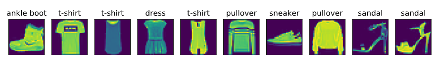
# 本函数已保存在d2lzh包中方便以后使用
def get_fashion_mnist_labels(labels):
    text_labels = ['t-shirt', 'trouser', 'pullover', 'dress', 'coat',
                   'sandal', 'shirt', 'sneaker', 'bag', 'ankle boot']
    return [text_labels[int(i)] for i in labels]
def show_fashion_mnist(images, labels):
    d2l.use_svg_display()
    # 这里的_表示我们忽略(不使用)的变量
    _, figs = plt.subplots(1, len(images), figsize=(12, 12))
    for f, img, lbl in zip(figs, images, labels):
        f.imshow(img.view((28, 28)).numpy())
        f.set_title(lbl)
        f.axes.get_xaxis().set_visible(False)
        f.axes.get_yaxis().set_visible(False)
    plt.show()
X, y = [], []
for i in range(10):
    X.append(mnist_train[i][0]) # 将第i个feature加到X中
    y.append(mnist_train[i][1]) # 将第i个label加到y中
show_fashion_mnist(X, get_fashion_mnist_labels(y))
softmax从零开始的实现
import torch
import torchvision
import numpy as np
import sys
sys.path.append("/home/kesci/input")
import d2lzh1981 as d2l

print(torch.__version__)
print(torchvision.__version__)
获取训练集数据和测试集数据
batch_size = 256
train_iter, test_iter = d2l.load_data_fashion_mnist(batch_size, root='/home/kesci/input/FashionMNIST2065')
模型参数初始化
num_inputs = 784
print(28*28)
num_outputs = 10

W = torch.tensor(np.random.normal(0, 0.01, (num_inputs, num_outputs)), dtype=torch.float)
b = torch.zeros(num_outputs, dtype=torch.float)
W.requires_grad_(requires_grad=True)
b.requires_grad_(requires_grad=True)
对多维Tensor按维度操作
X = torch.tensor([[1, 2, 3], [4, 5, 6]])
print(X.sum(dim=0, keepdim=True))  # dim为0,按照相同的列求和,并在结果中保留列特征
print(X.sum(dim=1, keepdim=True))  # dim为1,按照相同的行求和,并在结果中保留行特征
print(X.sum(dim=0, keepdim=False)) # dim为0,按照相同的列求和,不在结果中保留列特征
print(X.sum(dim=1, keepdim=False)) # dim为1,按照相同的行求和,不在结果中保留行特征
定义softmax操作
def softmax(X):
    X_exp = X.exp()
    partition = X_exp.sum(dim=1, keepdim=True)
    # print("X size is ", X_exp.size())
    # print("partition size is ", partition, partition.size())
    return X_exp / partition  # 这里应用了广播机制
X = torch.rand((2, 5))
X_prob = softmax(X)
print(X_prob, '\n', X_prob.sum(dim=1))
def net(X):
    return softmax(torch.mm(X.view((-1, num_inputs)), W) + b)
定义损失函数
y_hat = torch.tensor([[0.1, 0.3, 0.6], [0.3, 0.2, 0.5]])
y = torch.LongTensor([0, 2])
y_hat.gather(1, y.view(-1, 1))
def cross_entropy(y_hat, y):
    return - torch.log(y_hat.gather(1, y.view(-1, 1)))
定义准确率
def accuracy(y_hat, y):
    return (y_hat.argmax(dim=1) == y).float().mean().item()
# 本函数已保存在d2lzh_pytorch包中方便以后使用。该函数将被逐步改进:它的完整实现将在“图像增广”一节中描述
def evaluate_accuracy(data_iter, net):
    acc_sum, n = 0.0, 0
    for X, y in data_iter:
        acc_sum += (net(X).argmax(dim=1) == y).float().sum().item()
        n += y.shape[0]
    return acc_sum / n
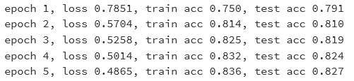
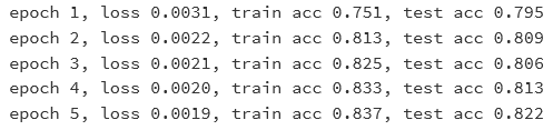
训练模型
num_epochs, lr = 5, 0.1
# 本函数已保存在d2lzh_pytorch包中方便以后使用
def train_ch3(net, train_iter, test_iter, loss, num_epochs, batch_size,
params=None, lr=None, optimizer=None):
for epoch in range(num_epochs):
train_l_sum, train_acc_sum, n = 0.0, 0.0, 0
for X, y in train_iter:
y_hat = net(X)
l = loss(y_hat, y).sum()
# 梯度清零
if optimizer is not None:
optimizer.zero_grad()
elif params is not None and params[0].grad is not None:
for param in params:
param.grad.data.zero_()
l.backward()
if optimizer is None:
d2l.sgd(params, lr, batch_size)
else:
optimizer.step()
train_l_sum += l.item()
train_acc_sum += (y_hat.argmax(dim=1) == y).sum().item()
n += y.shape[0]
test_acc = evaluate_accuracy(test_iter, net)
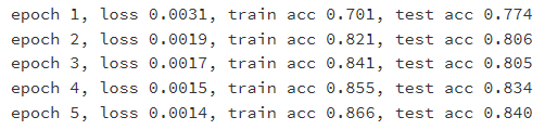
print('epoch %d, loss %.4f, train acc %.3f, test acc %.3f'
% (epoch + 1, train_l_sum / n, train_acc_sum / n, test_acc))
train_ch3(net, train_iter, test_iter, cross_entropy, num_epochs, batch_size, [W, b], lr)
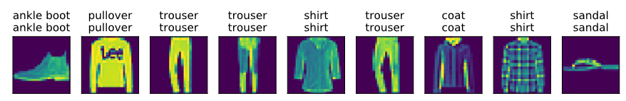
模型预测
X, y = iter(test_iter).next()

true_labels = d2l.get_fashion_mnist_labels(y.numpy())
pred_labels = d2l.get_fashion_mnist_labels(net(X).argmax(dim=1).numpy())
titles = [true + '\n' + pred for true, pred in zip(true_labels, pred_labels)]

d2l.show_fashion_mnist(X[0:9], titles[0:9])
softmax的简洁实现
# 加载各种包或者模块
import torch
from torch import nn
from torch.nn import init
import numpy as np
import sys
sys.path.append("/home/kesci/input")
import d2lzh1981 as d2l

print(torch.__version__)
batch_size = 256
train_iter, test_iter = d2l.load_data_fashion_mnist(batch_size, root='/home/kesci/input/FashionMNIST2065')
num_inputs = 784
num_outputs = 10

class LinearNet(nn.Module):
    def __init__(self, num_inputs, num_outputs):
        super(LinearNet, self).__init__()
        self.linear = nn.Linear(num_inputs, num_outputs)
    def forward(self, x): # x 的形状: (batch, 1, 28, 28)
        y = self.linear(x.view(x.shape[0], -1))
        return y

# net = LinearNet(num_inputs, num_outputs)

class FlattenLayer(nn.Module):
    def __init__(self):
        super(FlattenLayer, self).__init__()
    def forward(self, x): # x 的形状: (batch, *, *, ...)
        return x.view(x.shape[0], -1)

from collections import OrderedDict
net = nn.Sequential(
        # FlattenLayer(),
        # LinearNet(num_inputs, num_outputs)
        OrderedDict([
           ('flatten', FlattenLayer()),
           ('linear', nn.Linear(num_inputs, num_outputs))]) # 或者写成我们自己定义的 LinearNet(num_inputs, num_outputs) 也可以
        )
init.normal_(net.linear.weight, mean=0, std=0.01)
init.constant_(net.linear.bias, val=0)
loss = nn.CrossEntropyLoss() # 下面是他的函数原型
# class torch.nn.CrossEntropyLoss(weight=None, size_average=None, ignore_index=-100, reduce=None, reduction='mean')
optimizer = torch.optim.SGD(net.parameters(), lr=0.1) # 下面是函数原型
# class torch.optim.SGD(params, lr=, momentum=0, dampening=0, weight_decay=0, nesterov=False)
num_epochs = 5
d2l.train_ch3(net, train_iter, test_iter, loss, num_epochs, batch_size, None, None, optimizer)
第三部分:多层感知机
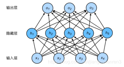

多层感知机从零开始的实现
import torch
import numpy as np
import sys
sys.path.append("/home/kesci/input")
import d2lzh1981 as d2l
print(torch.__version__)

batch_size = 256
train_iter, test_iter = d2l.load_data_fashion_mnist(batch_size,root='/home/kesci/input/FashionMNIST2065')

num_inputs, num_outputs, num_hiddens = 784, 10, 256

W1 = torch.tensor(np.random.normal(0, 0.01, (num_inputs, num_hiddens)), dtype=torch.float)
b1 = torch.zeros(num_hiddens, dtype=torch.float)
W2 = torch.tensor(np.random.normal(0, 0.01, (num_hiddens, num_outputs)), dtype=torch.float)
b2 = torch.zeros(num_outputs, dtype=torch.float)

params = [W1, b1, W2, b2]
for param in params:
    param.requires_grad_(requires_grad=True)

def relu(X):
    return torch.max(input=X, other=torch.tensor(0.0))

def net(X):
    X = X.view((-1, num_inputs))
    H = relu(torch.matmul(X, W1) + b1)
    return torch.matmul(H, W2) + b2

loss = torch.nn.CrossEntropyLoss()

num_epochs, lr = 5, 100.0
# def train_ch3(net, train_iter, test_iter, loss, num_epochs, batch_size,
#               params=None, lr=None, optimizer=None):
#     for epoch in range(num_epochs):
#         train_l_sum, train_acc_sum, n = 0.0, 0.0, 0
#         for X, y in train_iter:
#             y_hat = net(X)
#             l = loss(y_hat, y).sum()
#
#             # 梯度清零
#             if optimizer is not None:
#                 optimizer.zero_grad()
#             elif params is not None and params[0].grad is not None:
#                 for param in params:
#                     param.grad.data.zero_()
#
#             l.backward()
#             if optimizer is None:
#                 d2l.sgd(params, lr, batch_size)
#             else:
#                 optimizer.step()  # “softmax回归的简洁实现”一节将用到
#
#
#             train_l_sum += l.item()
#             train_acc_sum += (y_hat.argmax(dim=1) == y).sum().item()
#             n += y.shape[0]
#         test_acc = evaluate_accuracy(test_iter, net)
#         print('epoch %d, loss %.4f, train acc %.3f, test acc %.3f'
#               % (epoch + 1, train_l_sum / n, train_acc_sum / n, test_acc))

d2l.train_ch3(net, train_iter, test_iter, loss, num_epochs, batch_size, params, lr)
多层感知机pytorch实现
import torch
from torch import nn
from torch.nn import init
import numpy as np
import sys
sys.path.append("/home/kesci/input")
import d2lzh1981 as d2l

print(torch.__version__)

num_inputs, num_outputs, num_hiddens = 784, 10, 256

net = nn.Sequential(
        d2l.FlattenLayer(),
        nn.Linear(num_inputs, num_hiddens),
        nn.ReLU(),
        nn.Linear(num_hiddens, num_outputs),
        )

for params in net.parameters():
    init.normal_(params, mean=0, std=0.01)

batch_size = 256
train_iter, test_iter = d2l.load_data_fashion_mnist(batch_size,root='/home/kesci/input/FashionMNIST2065')
loss = torch.nn.CrossEntropyLoss()

optimizer = torch.optim.SGD(net.parameters(), lr=0.5)

num_epochs = 5
d2l.train_ch3(net, train_iter, test_iter, loss, num_epochs, batch_size, None, None, optimizer)