特征工程之特征选择（三）

特征工程之特征选择（三）

3.Embedded

3.1 基于L1正则(惩罚项)的特征选择

有过一点机器学习基础的同学都知道，将L1正则放置于cost function中，会起到特征选择的作用，它会使某些系数变为0,从而得到稀疏解，也起到一个降维的作用。
L1-norm:

$$\mid\mid{w}\mid\mid_1=\sum_i\mid{x_i}\mid$$
L2-norm: $$\mid\mid{w}\mid\mid_2=\sqrt{\sum_i{x_i^2}}$$
下面示例使用mse的cost function
L1正则的function： $$L(w)=\frac{1}{N}\sum_{i=1}^N(f(x_i;w)-y_i)+\lambda\mid\mid{w}\mid\mid_1$$
L2正则的function： $$L(w)=\frac{1}{N}\sum_{i=1}^N(f(x_i;w)-y_i)+\frac{\lambda}{2}\mid\mid{w}\mid\mid^2$$
至于为什么L1正则可以是的特征稀疏，详细推导过程我就不写了，只需要对w求偏导，再使用梯度下降优化更新就可以看出来
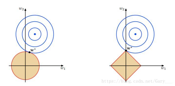
L1正则和L2正则的区别可以看下面这幅图，挺直观的，也是Andrew老师课上的图。

from sklearn.datasets import load_iris
from sklearn.svm import LinearSVC
from sklearn.feature_selection import SelectFromModel  # 使用SelectFromModel库来进行特征选择

# 导入数据
iris = load_iris()
X, y = iris.data, iris.target

# 查看数据的维度，可知道是一个有4维特征的数据
print(X.shape)

# 指定为l1正则项， C为惩罚系数，用来控制稀疏的程度，即在L1前面的系数，即alpha值，较小的C会导致少的特征被选择
lsvc = LinearSVC(penalty='l1', C=0.01, dual=False)  
lsvc.fit(X, y)
model = SelectFromModel(estimator=lsvc, prefit=True)# prefit=True,表示可使用训练的模型之后必须调用transform进行特征选择
X_new = model.transform(X)   # 进行特征选择
# 可以看出，移除掉了一个特征
print(X_new.shape)

下面是一个更加详细的例子

使用SelectFromModel和Lasso在Boston数据集中选择最好的特征

import matplotlib.pyplot as plt
import numpy as np

from sklearn.datasets import load_boston
from sklearn.linear_model import LassoCV
from sklearn.feature_selection import SelectFromModel

# 导入数据
boston = load_boston()
X, y = boston.data, boston.target

# 创建基础模型， 有同学会问道Lasso和LassoCV的区别，
# 区别就是后面的CV(Cross validation)一个用到交叉验证，一个没有
clf = LassoCV()

# 这里就使用到了一个参数为threshold(阈值)，即选择重要性大于该阈值的特征，其余的移除
sfm = SelectFromModel(estimator=clf, threshold=0.25)
sfm.fit(X, y)

# 进行特征选择，且返回筛选过后的特征维度,从结果来看，只剩下了5个特征(原本为13)
n_features = sfm.transform(X).shape[1]
print(n_features)

# 在这里，我们的目标是一直将模型训练，知道特征只剩两个
# 当前，我们需要一直增大threshold的强度，才能筛选出更少的特征
while n_features > 2 :
    sfm.threshold += 0.1
    X_transform = sfm.transform(X)
    n_features = X_transform.shape[1]
print(n_features)

# 画出特征
plt.title(
    "Features selected from Boston using SelectFromModel with "
    "threshold %0.3f.\n" % sfm.threshold)
feature_1 = X_transform[:, 0]
feature_2 = X_transform[:, 1]
plt.plot(feature_1, feature_2, 'r.')
plt.xlabel("Feature number 1")
plt.ylabel("Feature number 2")
plt.ylim([np.min(feature_2), np.max(feature_2)])
plt.show()

在这里强调一句，正则项的alpha数值不能随便乱选的，最好是通过交叉验证(LassoCV或LassoLarsCV)来寻找更优的alpha系数。

3.2 基于Tree(树)模型的特征选择

基于树的基类模型（有单树型sklearn.tree，也有树的森林sklearn.ensemble）可以用来计算特征的重要性，然后消除不相关的特征。

from sklearn.ensemble import ExtraTreesClassifier
from sklearn.datasets import load_iris
from sklearn.feature_selection import SelectFromModel

lris = load_iris()
X, y = lris.data, lris.target
print(X.shape)

clf = ExtraTreesClassifier()
clf = clf.fit(X, y)
# 查看特征重要性,可见后两个特征更为重要
print(clf.feature_importances_)

model = SelectFromModel(estimator=clf, prefit=True)
X_new = model.transform(X)
print(X_new.shape)

在小型人脸识别样例数据上的分类示例

import matplotlib.pyplot as plt

from sklearn.datasets import fetch_olivetti_faces
from sklearn.ensemble import ExtraTreesClassifier

# 导入数据,这个会自动从网上下载
data = fetch_olivetti_faces()
X_faces = data.images
y = data.target

print(X_faces.shape, len(set(y)))

# 我们取出前五类出来进行分析
plt.figure(figsize=(20, 20)) 
for i in range(5): 
    plt.subplot(1,5, i+1)
    plt.imshow(X_faces[i*10])
plt.show()

X = X_faces[0:50].reshape(len(X_faces[0:50]), -1)  # reshape成一维
y = y[0:50]
print(X.shape, y.shape)

%%time
# 创建一个带有1000棵树的森林
# 线程
n_jobs = 1
# 最佳分割时所要考虑的特征数量为128
forest = ExtraTreesClassifier(n_estimators=1000, max_features=128, n_jobs=n_jobs, random_state=0)
forest.fit(X, y)

importances = forest.feature_importances_
print(importances[:10])   # 输出前10个特征来看看
print(importances.shape)
importances = importances.reshape(X_faces[0].shape)
print(importances.shape)

# 画出像素重要性图案
plt.matshow(importances, cmap=plt.cm.Blues_r)
plt.title("Pixel importances with forests of trees\n")
plt.show()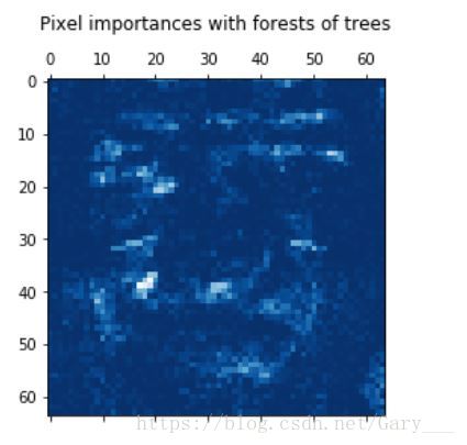

由上图可以看出，比较重要的特征都集中在人脸的五官的位置，人脸外的特征都不那么重要。

github地址，编文不易，欢迎star/follow：https://github.com/Gary-Deeplearning/sklearn-study-note