TinyMind人民币面值-热身赛
一、数据加载
# 加载标签
import numpy as np
import pandas as pd

label_path = "/home/jovyan/workspace/train_face_value_label -converted.csv"
df = pd.read_csv(label_path)
df_label = df.iloc[:,1]
label = np.array(df_label)
# 查看标签数据前10个数据
print(label[:10])
[8 7 0 5 8 6 3 0 0 1]
# 加载对应类别的金额
import pandas as pd

labelnames_file = "/home/jovyan/workspace/labelnames.csv"
labelnames = pd.read_csv(labelnames_file)
print(labelnames)
   classid  labelname
0        0        0.1
1        1        0.2
2        2        0.5
3        3        1.0
4        4        2.0
5        5        5.0
6        6       10.0
7        7       50.0
8        8      100.0
# 定义类别classid转换成labelname的函数
label_names = np.array(labelnames)
def id_to_name(id):
    return label_names[id][1]
# 加载训练集图片数据
# 读取图片数据
import numpy as np
import glob # 查找符合特定规则的文件路径名
from PIL import Image

train_image_path = "/home/jovyan/workspace/train_data/*.jpg"
train_data = np.zeros((39620,150,300,1))
i = 0
for imageFile in glob.glob(train_image_path):
    img_arr = np.array(Image.open(imageFile).convert("L")).reshape(150,300,1)
    train_data[i] = img_arr
    i += 1
# 划分训练集和验证集
x_train = train_data[:30000]
y_train = label[:30000]

x_valid = train_data[30000:]
y_valid = label[30000:]
二、探索数据集和标签
# 查看训练集的数量
print("the number of training examples:",x_train.shape[0])
# 查看测试集的数量
print("the number of valid examples:",x_valid.shape[0])
# 查看训练标签的数量
print("the number of training label:",len(y_train))
# 查看测试标签的数量
print("the number of valid label:",len(y_valid))
# 查看数据格式
print("the image data shape=",x_train.shape[1:])
the number of training examples: 30000
the number of valid examples: 9620
the number of training label: 30000
the number of valid label: 9620
the image data shape= (150, 300, 1)
# 查看数据标签的数量
import numpy as np

label_name = np.unique(y_train)
label_sum = len(label_name)

print("the labels is:",label_name)
print("the length of label is:",label_sum)
the labels is: [0 1 2 3 4 5 6 7 8]
the length of label is: 9
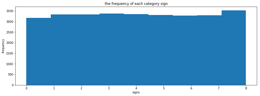
# 直方图来展示图像训练集的各个类别的分布情况
import matplotlib.pyplot as plt
%matplotlib inline
n_classes = len(np.unique(y_train))
def plot_y_train_hist():
    fig = plt.figure(figsize=(15,5))
    ax = fig.add_subplot(1,1,1)
    hist = ax.hist(y_train,bins = n_classes)
    ax.set_title("the frequency of each category sign")
    ax.set_xlabel("signs")
    ax.set_ylabel("frequency")
    plt.show()
    return hist

print(x_train.shape)
print(y_train.shape)
hist = plot_y_train_hist()
(30000, 150, 300, 1)
(30000,)
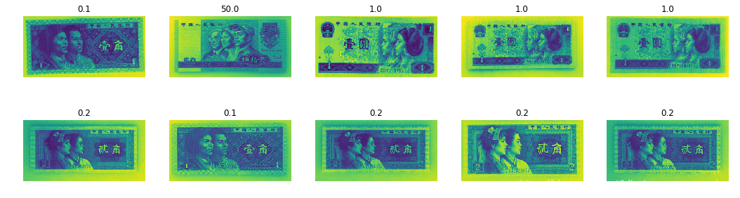
# 绘制money图
import matplotlib.pyplot as plt
%matplotlib inline

fig,axes = plt.subplots(2,5,figsize=(18,5))
ax_array = axes.ravel()
for ax in ax_array:
    index = np.random.randint(0,len(x_train))
    ax.imshow(x_train[index].reshape(150,300))
    ax.axis("off")
    ax.set_title(id_to_name(y_train[index]))
plt.show()
三、数据集中处理
# 图像数据归一化处理
x_train = np.array(x_train,dtype=np.float32)
x_valid = np.array(x_valid,dtype=np.float32)
X_train = (x_train-128)/128
X_valid = (x_valid-128)/128
print(X_train[0])
[[[ 0.8203125]
  [ 0.8203125]
  [ 0.8125   ]
  ...,
  [ 0.78125  ]
  [ 0.7890625]
  [ 0.8046875]]

 [[ 0.8203125]
  [ 0.8203125]
  [ 0.8203125]
  ...,
  [ 0.78125  ]
  [ 0.7890625]
  [ 0.8046875]]

 [[ 0.8203125]
  [ 0.8203125]
  [ 0.8203125]
  ...,
  [ 0.78125  ]
  [ 0.7890625]
  [ 0.8046875]]

 ...,
 [[ 0.9609375]
  [ 0.9609375]
  [ 0.96875  ]
  ...,
  [ 0.9296875]
  [ 0.9296875]
  [ 0.9296875]]

 [[ 0.9609375]
  [ 0.9609375]
  [ 0.96875  ]
  ...,
  [ 0.9375   ]
  [ 0.9375   ]
  [ 0.9375   ]]

 [[ 0.9609375]
  [ 0.9609375]
  [ 0.96875  ]
  ...,
  [ 0.9375   ]
  [ 0.9453125]
  [ 0.9453125]]]
print(X_train.shape,type(X_train))
print(X_valid.shape,type(X_valid))
(30000, 150, 300, 1) <class 'numpy.ndarray'>
(9620, 150, 300, 1) <class 'numpy.ndarray'>
# 标签数据one-hot编码处理
from tensorflow import keras
from keras.utils import np_utils
print("Shape before one-hot encoding:",y_train.shape)
Y_train = np_utils.to_categorical(y_train,label_sum)
Y_valid = np_utils.to_categorical(y_valid,label_sum)
print("Shape after one-hot encoding:",Y_train.shape)
print("Shape after one-hot encoding:",Y_valid.shape)
Shape before one-hot encoding: (30000,)
Shape after one-hot encoding: (30000, 9)
Shape after one-hot encoding: (9620, 9)


Using TensorFlow backend.
四、模型的建立
from keras.models import Sequential
from keras.layers import Dense,Dropout,Flatten
from keras.layers import Conv2D,MaxPooling2D

model = Sequential()

# layers1
model.add(Conv2D(filters=32,
                 kernel_size=(3,3),
                 input_shape=X_train.shape[1:],
                 activation="relu"))
model.add(MaxPooling2D(pool_size=(2,2)))

model.add(Dropout(0.5))


# layers2
model.add(Conv2D(filters=32,
                 kernel_size=(3,3),
                 activation="relu"))
model.add(MaxPooling2D(pool_size=(2,2)))

model.add(Dropout(0.5))

# layers3
model.add(Conv2D(filters=32,
                 kernel_size=(3,3),
                 activation="relu"))
model.add(MaxPooling2D(pool_size=(2,2)))

model.add(Dropout(0.5))


# flattern
model.add(Flatten())

# Dense
model.add(Dense(label_sum,activation="softmax"))
# 查看模型结构
model.summary()
_________________________________________________________________
Layer (type)                 Output Shape              Param #
=================================================================
conv2d_1 (Conv2D)            (None, 148, 298, 32)      320
_________________________________________________________________
max_pooling2d_1 (MaxPooling2 (None, 74, 149, 32)       0
_________________________________________________________________
dropout_1 (Dropout)          (None, 74, 149, 32)       0
_________________________________________________________________
conv2d_2 (Conv2D)            (None, 72, 147, 32)       9248
_________________________________________________________________
max_pooling2d_2 (MaxPooling2 (None, 36, 73, 32)        0
_________________________________________________________________
dropout_2 (Dropout)          (None, 36, 73, 32)        0
_________________________________________________________________
conv2d_3 (Conv2D)            (None, 34, 71, 32)        9248
_________________________________________________________________
max_pooling2d_3 (MaxPooling2 (None, 17, 35, 32)        0
_________________________________________________________________
dropout_3 (Dropout)          (None, 17, 35, 32)        0
_________________________________________________________________
flatten_1 (Flatten)          (None, 19040)             0
_________________________________________________________________
dense_1 (Dense)              (None, 9)                 171369
=================================================================
Total params: 190,185
Trainable params: 190,185
Non-trainable params: 0
_________________________________________________________________
# 编译模型
model.compile(loss="categorical_crossentropy",
              metrics=["accuracy"],
              optimizer="adam")
# 训练模型
history = model.fit(X_train,
                    Y_train,
                    batch_size=50,
                    epochs=5,
                    verbose=2,
                    validation_data=(X_valid,Y_valid))
Train on 30000 samples, validate on 9620 samples
Epoch 1/5
 - 65s - loss: 0.0561 - acc: 0.9846 - val_loss: 0.0131 - val_acc: 0.9988
Epoch 2/5
 - 61s - loss: 0.0146 - acc: 0.9985 - val_loss: 0.0109 - val_acc: 0.9993
Epoch 3/5
 - 61s - loss: 0.0105 - acc: 0.9993 - val_loss: 0.1261 - val_acc: 0.9598
Epoch 4/5
 - 60s - loss: 0.0191 - acc: 0.9981 - val_loss: 0.2859 - val_acc: 0.9885
Epoch 5/5
 - 60s - loss: 0.0120 - acc: 0.9989 - val_loss: 0.0092 - val_acc: 0.9992
# 保存模型
import os
import tensorflow.gfile as gfile

save_dir = "/home/jovyan/workspace/mondel/"

if gfile.Exists(save_dir):
    gfile.DeleteRecursively(save_dir)
gfile.MakeDirs(save_dir)

model_name = 'keras_money_v1.h5'
model_path = os.path.join(save_dir, model_name)
model.save(model_path)
print('Saved trained model at %s ' % model_path)
Saved trained model at /home/jovyan/workspace/mondel/keras_money_v1.h5
五、预测数据
1.待预测数据导入并保存图片名称
# 保存图片名称
import os
import numpy as np
test_image_path = "/home/jovyan/workspace/test_data/"
write_file_name = "/home/jovyan/workspace/name.txt"
test_image_list = []

for image_name in os.listdir(test_image_path):
    test_image_list.append(image_name)
number_of_lines = len(test_image_list)
print(number_of_lines)
20000
# 写入txt文件中,逐行写入
write_file = open(write_file_name,"w")
for current_line in range(number_of_lines):
    write_file.write(test_image_list[current_line]+"\n")
# 关闭文件
write_file.close()
********* 分割线 *********
# 加载预测数据
import numpy as np
import glob
from PIL import Image

test_image_path = "/home/jovyan/workspace/test_data/*.jpg"
test_data = np.zeros((20000,150,300,1))


i = 0
for imageFile in glob.glob(test_image_path):
    img_arr = np.array(Image.open(imageFile).convert("L")).reshape(150,300,1)

    test_data[i] = img_arr
    i += 1
# 查看测试集的数量
print("the number of training examples:",test_data.shape[0])

# 查看数据格式
print("the image data shape=",test_data.shape[1:])
the number of training examples: 20000
the image data shape= (150, 300, 1)
2.带预测数据预处理
x_test = np.array(test_data,dtype=np.float32)
X_test = (x_test-128)/128
print(X_test.shape,type(X_test))
(20000, 150, 300, 1) <class 'numpy.ndarray'>
3.模型对待预测数据预测
# 对带预测数据进行一寸
res = model.predict_classes(X_test)
# 查看预测结果前10个
print(res[:10])
[2 4 6 1 3 3 1 2 6 1]
# 查看预测结果的类型
print(res.shape,type(res))
(20000,) <class 'numpy.ndarray'>
# id转金额
res_converted = np.zeros((20000))
for i in range(len(res)):
    res_converted[i] = id_to_name(res[i])
# 查看预测结果转换金额后的前10个
print(res_converted[:10])
[ 0.5 2. 10. 0.2 1. 1. 0.2 0.5 10. 0.2]
print(res_converted.shape,type(res_converted))
(20000,) <class 'numpy.ndarray'>
# 将预测值保存至txt文档中
import numpy as np
np.savetxt("res.txt",res_converted,fmt='%.1f')
