题目
在这部分的练习中,你将建立一个逻辑回归模型来预测一个学生是否能进入大学。假设你是一所大学的行政管理人员,你想根据两门考试的结果,来决定每个申请人是否被录取。你有以前申请人的历史数据,可以将其用作逻辑回归训练集。对于每一个训练样本,你有申请人两次测评的分数以及录取的结果。为了完成这个预测任务,我们准备构建一个可以基于两次测试评分来评估录取可能性的分类模型。
编程实现
1.Visualizing the data
在开始实现任何学习算法之前,如果可能的话,最好将数据可视化。
import numpy as np
import pandas as pd
import matplotlib.pyplot as plt


data = pd.read_csv('D:\BaiduNetdiskDownload\data_sets\ex2data1.txt', names=['exam1', 'exam2', 'admitted'])
data.head()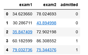
# 把数据分成 positive 和 negetive 两类
positive = data[data.admitted.isin(['1'])]  # admitted=1 为 positive 类
negetive = data[data.admitted.isin(['0'])]  # admitted=0 为 negetive 类

fig, ax = plt.subplots(figsize=(8,7))
ax.scatter(positive['exam1'], positive['exam2'], c='b', label='Admitted')
ax.scatter(negetive['exam1'], negetive['exam2'], s=50, c='r', marker='x', label='Not Admitted') # s 设置点的大小;marker 设置画图的形状


#设置图例在右上角
# ax.legend(loc=1)


# 设置图例显示在图的上方
box = ax.get_position()
ax.set_position([box.x0, box.y0, box.width , box.height* 0.8])
ax.legend(loc='center left', bbox_to_anchor=(0.2, 1.12),ncol=3)


# 设置横纵坐标名
ax.set_xlabel('Exam 1 Score')
ax.set_ylabel('Exam 2 Score')
plt.show()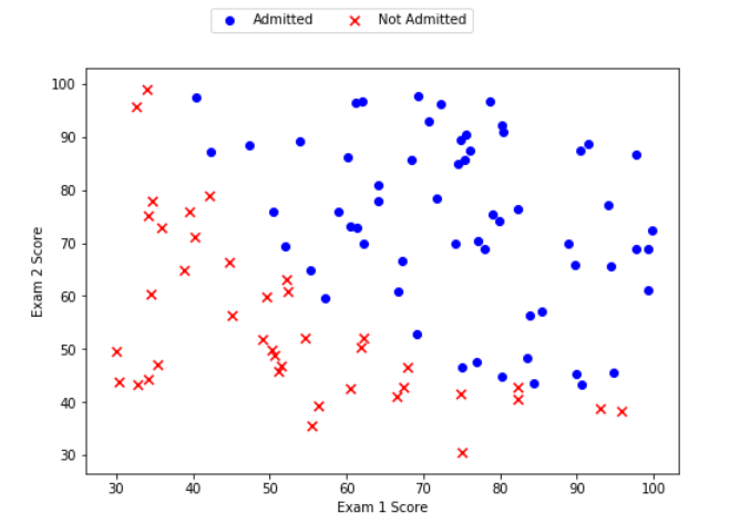
可以看到在两类间,有一个清晰的决策边界。现在我们需要实现逻辑回归,那样就可以训练一个模型来预测结果。
2.Sigmoid function
首先来回顾下 logistic 回归的假设函数:
\[ h_{\theta}\left(x\right)=g\left( \theta^T x \right)=\frac{1}{1+e^{-\theta^T x } } \]
令 \(\theta^T x = z\),其中,\(g(z)\) 被称为 Sigmoid function (S型函数)或 Logistic function:
\[ g(z)=\frac{1}{1+e^{-z}} \]
def sigmoid(z):
    return 1 / (1 + np.exp(- z))

x1 = np.arange(-10, 10, 0.1)
plt.plot(x1, sigmoid(x1), c='r')
plt.show()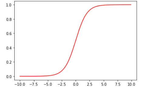
3.Cost function
逻辑回归的代价函数如下:
\[ J(\theta)=\frac1m \sum_{i=1}^m \left( - y^{\left(i \right)} log \left( h_\theta \left( x^{\left( i\right)} \right) \right) - \left( 1-y^{\left( i\right)} \right) log \left( 1- h_\theta \left( x^{\left( i\right)} \right) \right) \right) \]
\[ h_{\theta}\left(x\right)=g\left( \theta^T x \right) \]
# 定义代价函数(能够返回代价函数值)
def cost(theta, X, y):
    first = (-y) * np.log(sigmoid(X @ theta)) # 注意这里的 theta 是列向量
    second = (1 - y)*np.log(1 - sigmoid(X @ theta))
    return np.mean(first - second)
# add a ones column - this makes the matrix multiplication work out easier
if 'Ones' not in data.columns:
data.insert(0, 'Ones', 1)
# set X (training data) and y (target variable)
# 用.iloc来取列
X = data.iloc[:, :-1].values # Convert the frame to its Numpy-array representation.
y = data.iloc[:, -1].values # Return is NOT a Numpy-matrix, rather, a Numpy-array.
theta = np.zeros(X.shape[1]) # X.shape[1]获取X的列数,这里theta是列向量检查矩阵的维度:
X.shape, theta.shape, y.shape
计算代价函数的初始值:
cost(theta, X, y)
接下来,我们需要一个函数来计算我们的训练数据、标签和一些参数thate的梯度。
4.Gradient
计算梯度值:
\[ \frac{\partial }{\partial \theta_j} J(\theta)=\frac1m \sum_{i=1}^m \left( h_\theta \left( x^{ \left(i\right) } \right) -y{ \left(i\right) } \right) x_{j}^{\left(i\right)} \]
转化为向量化计算:
\[ \frac1m X^T\left( sigmoid\left( X \theta \right)-y\right) \]
在此题中 ,\(X\) 是100*3的矩阵, \(X^T\) 就是3*100的矩阵。\(\theta\) 是3*1的矩阵,则最后求得的梯度值是一个3*1的矩阵。
# 定义计算梯度值(导数值)
def gradient(theta, X, y):
    return (X.T @ (sigmoid(X @ theta) - y))/len(X)
# the gradient of the cost is a vector of the same length as θ where the jth element (for j = 0, 1, . . . , n)
计算梯度值的初始数据:
gradient(theta, X, y)
注意,我们还没有在执行梯度下降算法,这里仅仅在计算梯度值。
5.Learning θ parameters
- 在视频中,一个称为“fminunc”的Octave函数是用来优化函数来计算成本和梯度参数。
- 由于我们使用Python,我们可以用SciPy的“optimize”命名空间来做同样的事情。
这里我们使用的是高级优化算法,运行速度通常远远超过梯度下降。方便快捷。
只需传入cost函数,已经所求的变量theta,和梯度。注意:cost函数定义变量时变量theta要放在第一个,若cost函数只返回cost,则设置fprime=gradient。
import scipy.optimize as opt

# 这里使用fimin_tnc方法来拟合
result = opt.fmin_tnc(func=cost, x0=theta, fprime=gradient, args=(X, y))

result
计算优化算法之后的代价值函数值:
cost(result[0], X, y)
6.Evaluating logistic regression
- 学习好了参数\(θ\)后,我们来用这个模型预测某个学生是否能被录取。
- 接下来,我们需要编写一个函数,用我们所学的参数\(\theta\)来为数据集\(X\)输出预测。然后,我们可以使用这个函数来给我们的分类器的训练精度打分。
- 逻辑回归模型的假设函数:
\[ h_{\theta}\left(x\right)=\frac{1}{1+e^{-\theta^T x } } \] - 当\({h}_{\theta }\)大于等于0.5时,预测 y=1
- 当\({h}_{\theta }\)小于0.5时,预测 y=0
def predict(theta, X):
    probability = sigmoid(X @ theta)
    return [1 if x >= 0.5 else 0 for x in probability]  # return a list
final_theta = result[0]
predictions = predict(final_theta, X)
correct = [1 if a==b else 0 for (a, b) in zip(predictions, y)]
accuracy = sum(correct) / len(X)
accuracy
可以看到预测精度达到了89%。
7.Decision boundary(决策边界)
决策边界:
\[ \theta^T x=0 \]
此题中决策边界为:
\[ \theta_0+\theta_1x_1+\theta_2x_2=0 \]
x1 = np.arange(130, step=0.1)
x2 = -(final_theta[0] + x1*final_theta[1]) / final_theta[2]


fig, ax = plt.subplots(figsize=(8,5))
ax.scatter(positive['exam1'], positive['exam2'], c='b', label='Admitted')
ax.scatter(negetive['exam1'], negetive['exam2'], s=50, c='r', marker='x', label='Not Admitted')
ax.plot(x1, x2)
ax.set_xlim(0, 130)
ax.set_ylim(0, 130)
ax.set_xlabel('x1')
ax.set_ylabel('x2')
ax.set_title('Decision Boundary')
plt.show()
总结
逻辑回归的实现需要自己编写计算cost和gradient的函数,然后通过高级的优化算法就可以得到theta的最优解,不需要自己手动编写梯度下降函数。高级的优化算法不需要手动选择学习率α,收敛的速度远远快于梯度下降,但是要比梯度下降复杂。线性回归可以使用高级优化算法吗?明天试一下。