循环神经网络让神经网络有了记忆, 对于序列话的数据,循环神经网络能达到更好的效果.
我们将图片数据看成一个时间上的连续数据, 每一行的像素点都是这个时刻的输入, 读完整张图片就是从上而下的读完了每行的像素点. 然后我们就可以拿出 RNN 在最后一步的分析值判断图片是哪一类了
下面,我们手写数字的RNN
RNN和LSTM网络
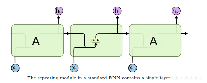
标准RNN模型
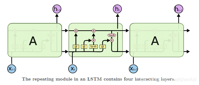
LSTM 模型
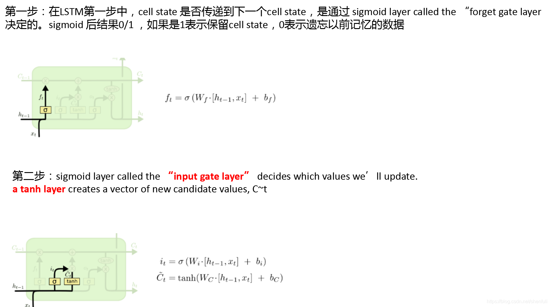
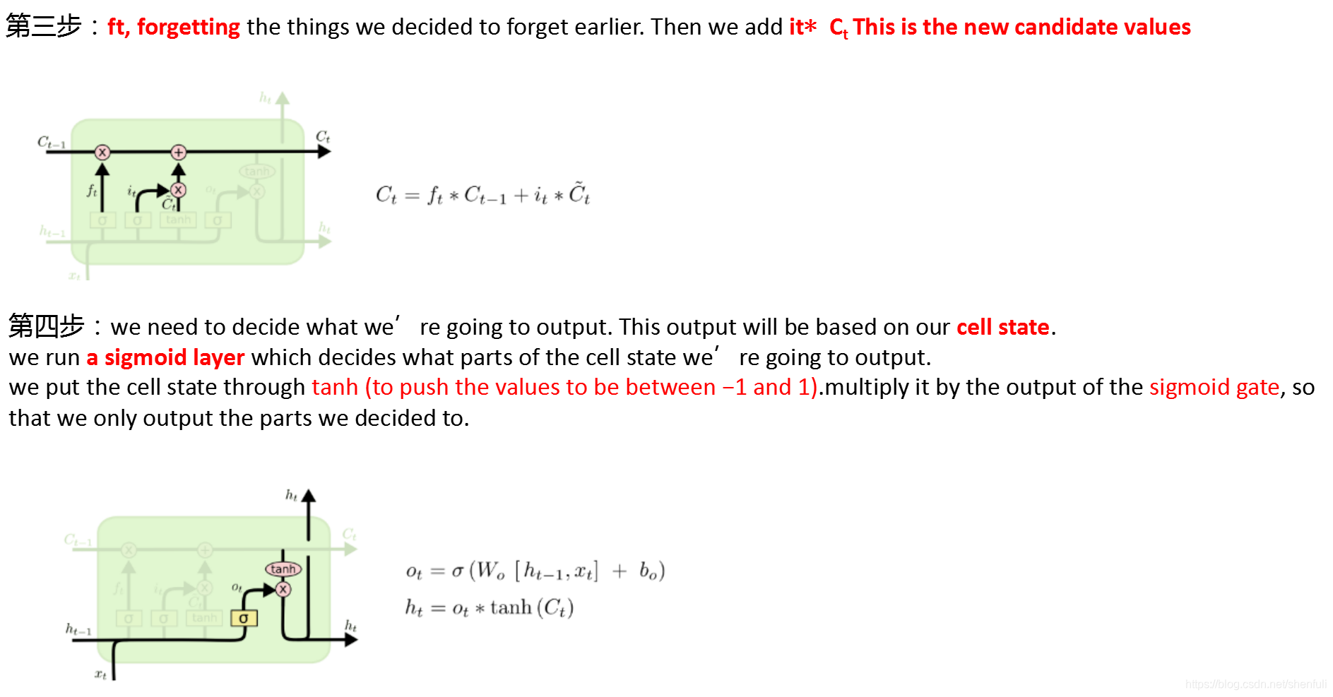
通过每步分析LSTM网络

导入库
import torch
from torch import nn
import torchvision.datasets
import torchvision.transforms as transforms
import matplotlib.pyplot as plt
import warnings
warnings.filterwarnings('ignore')
torch.manual_seed(1)    # reproducible
定义超参数
input_x就是图片中输入X的序列,相当于每一个输入X,都是1×28的大小,time_steps就是图片中绿色框的个数,图中用A表示的,也就是说总共有28个,因为图像是28×28
# Hyper Parameters
EPOCH = 1           # 训练整批数据多少次, 为了节约时间, 我们只训练一次
BATCH_SIZE = 64
TIME_STEP = 28      # rnn 时间步数 / 图片高度 (因为每张图像为28×28,而每一个序列长度为1×28,所以总共28个1×28,)
INPUT_SIZE = 28     # rnn 每步输入值 / 图片每行像素(输入序列的长度,因为是28×28的大小,所以每一个序列我们设置长度为28,每一个输入都是28个像素点)
LR = 0.01           # learning rate
DOWNLOAD_MNIST = True  # 如果你已经下载好了mnist数据就写上 Fasle

NUM_CLASSES = 10 #输入为10,因为共10类
HIDDEN_SIZE = 128 #隐层的大小,这个参数就是比如我们输入是1×28的矩阵大小,隐藏为128,就是将输入维度变为1×128,当然lstm输入也是1×128
训练和测试数据定义
# Mnist 手写数字
train_data = torchvision.datasets.MNIST(
    root='./mnist/',    # 保存或者提取位置
    train=True,  # this is training data
    transform=torchvision.transforms.ToTensor(),    # 转换 PIL.Image or numpy.ndarray 成
                                                    # torch.FloatTensor (C x H x W), 训练的时候 normalize 成 [0.0, 1.0] 区间
    download=DOWNLOAD_MNIST,          # 没下载就下载, 下载了就不用再下了
)

# plot one example
print(train_data.train_data.size())     # (60000, 28, 28)
print(train_data.train_labels.size())   # (60000)
plt.imshow(train_data.train_data[0].numpy(), cmap='gray')
plt.title('MNIST:%i' % train_data.train_labels[0])
plt.show()


输入内容:
torch.Size([60000, 28, 28])
torch.Size([60000])
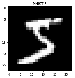
黑色的地方的值都是0, 白色的地方值大于0.
同样, 我们除了训练数据, 还给一些测试数据, 测试看看它有没有训练好.
# Data Loader for easy mini-batch return in training
train_loader = torch.utils.data.DataLoader(dataset=train_data, batch_size=BATCH_SIZE, shuffle=True)

data = next(iter(train_loader))
print(data[0].shape)#torch.Size([64, 1, 28, 28])
print(data[1].shape)#torch.Size([64])


for step, (b_x, b_y) in enumerate(train_loader):        # gives batch data
        b_x = b_x.view(-1, 28, 28)              # reshape x to (batch, time_step, input_size) => torch.Size([64, 28, 28])
        print(b_x.shape)#torch.Size([64, 28, 28])
        print(b_y.shape)#torch.Size([64])

        print(b_x[0].shape)#torch.Size([28, 28])
        print(b_y[0])#tensor(9)
        break

test_data = torchvision.datasets.MNIST(root='./mnist/', train=False, transform=transforms.ToTensor())
test_x = test_data.test_data.type(torch.FloatTensor)[:2000]/255.   # shape (2000, 28, 28) value in range(0,1)
test_y = test_data.test_labels.numpy()[:2000]    # covert to numpy array
print(test_x.shape) # torch.Size([2000, 28, 28])
定义RNN模型
用一个 class 来建立 RNN 模型. 这个 RNN 整体流程是
(input0, state0) -> LSTM -> (output0, state1);
(input1, state1) -> LSTM -> (output1, state2);
…
(inputN, stateN)-> LSTM -> (outputN, stateN+1);
outputN -> Linear -> prediction. 通过LSTM分析每一时刻的值, 并且将这一时刻和前面时刻的理解合并在一起, 生成当前时刻对前面数据的理解或记忆.
class RNN(nn.Module):
    def __init__(self):
        super(RNN, self).__init__()

        self.rnn = nn.LSTM(     # LSTM 效果要比 nn.RNN() 好多了
            input_size=INPUT_SIZE,      # 图片每行的数据像素点
            hidden_size=HIDDEN_SIZE,     # rnn hidden unit
            num_layers=1,       # 有几层 RNN layers
            batch_first=True,   # input & output 会是以 batch size 为第一维度的特征集 e.g. (batch, time_step, input_size)
        )

        self.out = nn.Linear(HIDDEN_SIZE, NUM_CLASSES)    # 输出层

    def forward(self, x):
        # x shape (batch, time_step, input_size)
        # r_out shape (batch, time_step, output_size)
        # h_n shape (n_layers, batch, hidden_size)   LSTM 有两个 hidden states, h_n 是分线, h_c 是主线
        # h_c shape (n_layers, batch, hidden_size)
        r_out, (h_n, h_c) = self.rnn(x, None)   # None 表示 hidden state 会用全0的 state

        # 这个地方选择lstm_output[-1],也就是相当于最后一个输出,因为其实每一个cell(相当于图中的A)都会有输出,但是我们只关心最后一个
        # 选取最后一个时间点的 r_out 输出
        # 这里 r_out[:, -1, :] 的值也是 h_n 的值
        out = self.out(r_out[:, -1, :]) # torch.Size([64, 28, 64])-> torch.Size([64, 10])
        return out

rnn = RNN()
print(rnn)
输出结果:
RNN(
(rnn): LSTM(28, 128, batch_first=True)
(out): Linear(in_features=128, out_features=10, bias=True)
)
RNN模型训练和预测
我们将图片数据看成一个时间上的连续数据, 每一行的像素点都是这个时刻的输入, 读完整张图片就是从上而下的读完了每行的像素点. 然后我们就可以拿出 RNN 在最后一步的分析值判断图片是哪一类了
optimizer = torch.optim.Adam(rnn.parameters(), lr=LR)   # optimize all cnn parameters
loss_func = nn.CrossEntropyLoss()                       # the target label is not one-hotted

# training and testing
for epoch in range(EPOCH):
    for step, (b_x, b_y) in enumerate(train_loader):        # gives batch data
        b_x = b_x.view(-1, 28, 28)                      # reshape x to (batch, time_step, input_size) => torch.Size([64, 28, 28])

        output = rnn(b_x)                               # rnn output
        loss = loss_func(output, b_y)                   # cross entropy loss
        optimizer.zero_grad()                           # clear gradients for this training step
        loss.backward()                                 # backpropagation, compute gradients
        optimizer.step()                                # apply gradients

        if step % 50 == 0:
            test_output = rnn(test_x)                   # (samples, time_step, input_size)
            pred_y = torch.max(test_output, 1)[1].data.numpy()
            accuracy = float((pred_y == test_y).astype(int).sum()) / float(test_y.size)
            print('Epoch: ', epoch, '| train loss: %.4f' % loss.data.numpy(), '| test accuracy: %.2f' % accuracy)
打印LOG日志数据如下:
Epoch:  0 | train loss: 2.2991 | test accuracy: 0.10
Epoch:  0 | train loss: 1.3363 | test accuracy: 0.54
Epoch:  0 | train loss: 0.7343 | test accuracy: 0.73
Epoch:  0 | train loss: 0.2725 | test accuracy: 0.82
Epoch:  0 | train loss: 0.7002 | test accuracy: 0.87
Epoch:  0 | train loss: 0.2219 | test accuracy: 0.89
Epoch:  0 | train loss: 0.1839 | test accuracy: 0.92
Epoch:  0 | train loss: 0.2430 | test accuracy: 0.90
Epoch:  0 | train loss: 0.0376 | test accuracy: 0.92
Epoch:  0 | train loss: 0.1351 | test accuracy: 0.94
Epoch:  0 | train loss: 0.1147 | test accuracy: 0.95
Epoch:  0 | train loss: 0.1830 | test accuracy: 0.93
Epoch:  0 | train loss: 0.2644 | test accuracy: 0.94
Epoch:  0 | train loss: 0.0898 | test accuracy: 0.95
Epoch:  0 | train loss: 0.1740 | test accuracy: 0.95
Epoch:  0 | train loss: 0.1634 | test accuracy: 0.94
Epoch:  0 | train loss: 0.1910 | test accuracy: 0.96
Epoch:  0 | train loss: 0.2034 | test accuracy: 0.95
Epoch:  0 | train loss: 0.1114 | test accuracy: 0.96
最后我们再来取10个数据, 看看预测的值到底对不对:
# print 10 predictions from test data
test_output = rnn(test_x[:10].view(-1, 28, 28))
pred_y = torch.max(test_output, 1)[1].data.numpy()
print(pred_y, 'prediction number')
print(test_y[:10], 'real number')
最终预测结果
torch.Size([10, 28, 64])
torch.Size([10, 10])
[8 8 8 8 8 8 8 8 8 8] prediction number
tensor([7, 2, 1, 0, 4, 1, 4, 9, 5, 9]) real number
更多资料请关注: https://github.com/shenfuli/ai
