- 绘图结果不可赋给一个对象,而是直接输出到一个“绘图设备”上,而绘图设备是一个绘图的窗口或是文件
- 绘图函数分为:高级绘图函数和低级绘图函数。其中,高级绘图函数创建新图形,而低级绘图函数在现存的图形上添加元素。
- 绘图参数控制绘图选项,可以使用缺省值,或是使用函数par修改。
- 打开绘图窗口使用命令
x11()或是windows(). - 打开文件作为绘图设备,包括
postscript()orpdf()orpng()。使用?device查看绘图列表。 - 最后打开的设备是当前的绘图设备。使用
dev.list()显示打开的列表。
> dev.list()
windows     pdf windows
      2       3       4 #数字是设备的编号
> dev.cur() #查看当前设备
windows
      4
> dev.set(3)  #把当前设备设置为编号为3的绘图设备
pdf
  3
> dev.off(3)  #关闭3号绘图设备
windows #返回:关闭后的当前设备
      4
> dev.off() #缺省,即关闭当前设备
windows #返回:关闭后的当前设备
      2
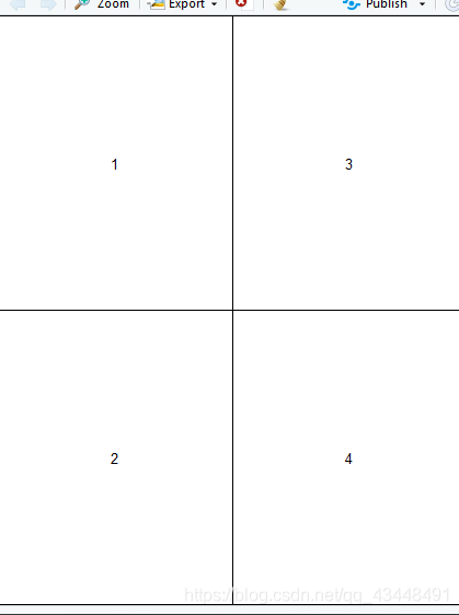
分割图形窗口,使用layout:
layout(matrix(1:4 , 2 , 2))
layout.show(4)#参数4表示展示出4个图形子窗口
#又如
layout(matrix(1:6 , 2 , 3))
layout.show(6)
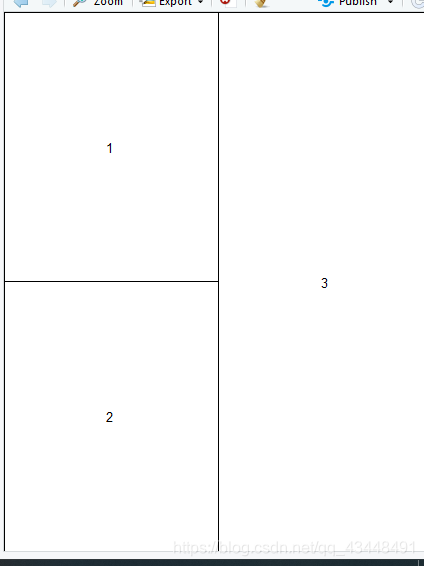
> m <- matrix(c(1:3 , 3) , 2 , 2)
> layout(m)
> layout.show(3)
>
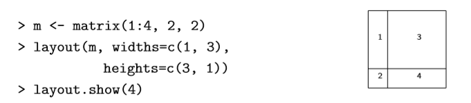
使用layout()等间距分配子窗口;
或是使用选项widths或是heights,如下:
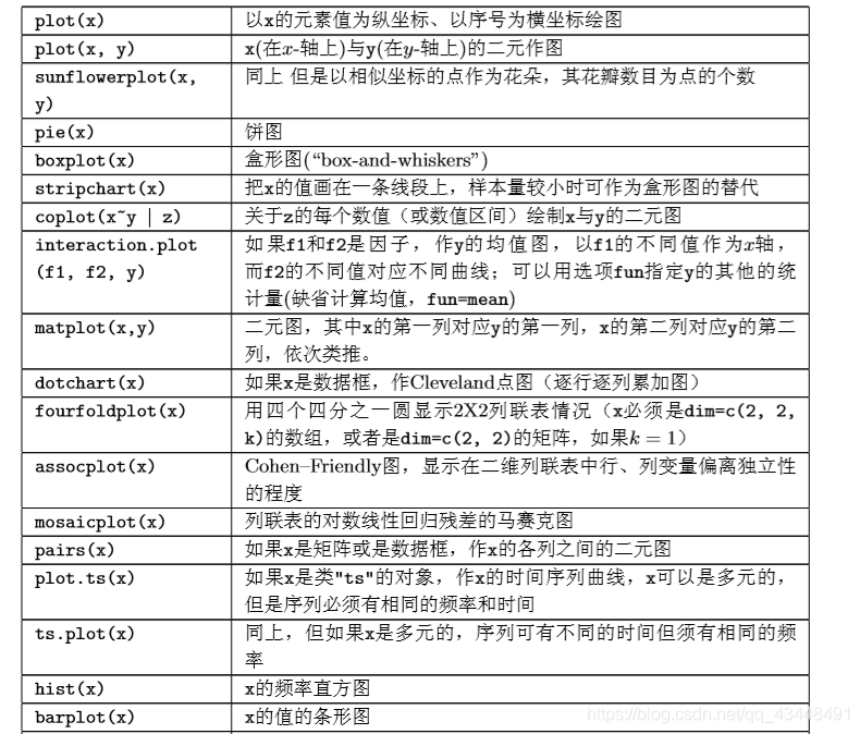
高级绘图函数

绘图过程中的一些共同选项及其缺省值:
add = FALSE,需要叠加图形到前一个图形中去么?
axes = TRUE , 需要绘制轴与边框么?
type = "p" , 指定图形的类型,“p”:点; “l”:线; “b":点连线 ; “o”:点连线,但是线在点上; “h”:垂直线; “s”:阶梯式,垂直线顶端显示数据;
xlim = ,ylim =指定轴的上下限,例如xlim=c(1,10),或是x =range(x)
xlab = ,ylab =坐标轴标签,必须是字符型值
main =主标题,必须是字符型值
sub =副标题,用小字体
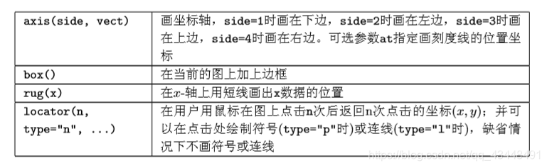
低价绘图命令:
作用于现存的图形上。
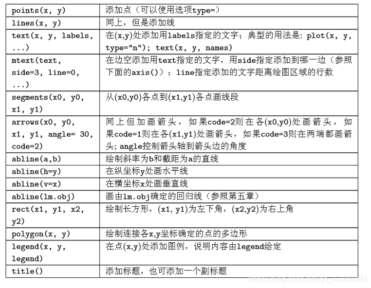
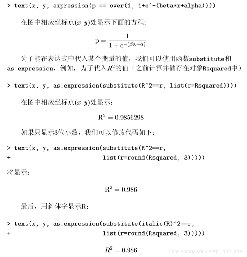
使用text()函数添加数学公式
text(x , y , expression( ……)在图形上添加数学公式,函数expression()把自变量转化为数学公式。
par()函数永久地改编绘图参数
永久地,也就是之后的图形都会按照par指定的参数来绘制图形。
当然也可以在绘图函数中修改。
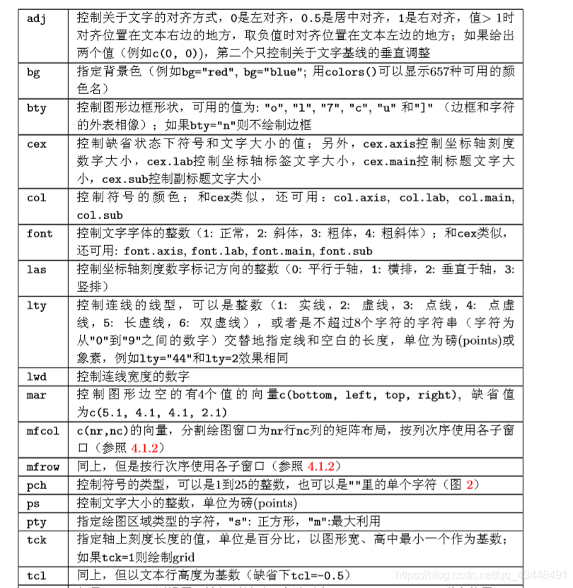
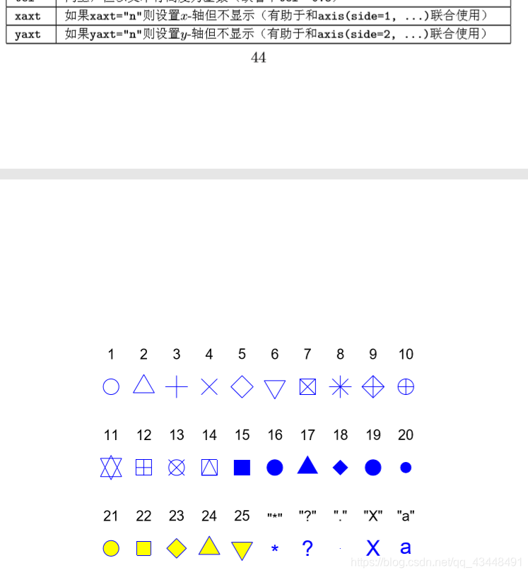
也可使用任意字符作为绘点符号:pch = “*”,"?"…
因为对par函数中的选项是永久性的,为了方便恢复,应该预先保存它的初始值以便以后恢复使用。
> par(bg = "lightyellow" , col.axis = "blue" , mar = c(4,  4, 2.5, 0.25))
> plot(x,y , xlab = "Ten random values" , ylab = "Ten other values" , xlim = c(-2 , 2) , ylim = c(-2 , 2) , pch = 22 , col = "red" , bg = "yellow" , bty = "l" , tcl =0.1 , main = "customizee a plot with R" , las =1 , cex = 1.5)
> par(opar) #恢复初始的绘图参数
#完全控制绘图案例
opar <- par()
par(bg = "lightyellow" , col.axis = "blue" , mar = c(4,  4, 2.5, 0.25))
plot(x, y, type = "n" , xlab="", ylab="", xlim = c(-2 , 2) , ylim = c(-2 , 2) , xaxt = "n"  , yaxt = "n")#type= "n"表示不画出点;最后两个参数xaxt,yaxt表示不画坐标轴,也可使用axes = FALSE(无坐标轴,也无边框)
rect(-3 , -3 , 3 , 3 , col = "cornsilk")#修改绘图趋于颜色,和区域大小
points(x , y , pch = 10 , col = "red" , cex = 2)#画点
axis(side = 1, c(-2 , 0 , 2) , tcl = -0.2 , labels = FALSE)
axis(side = 2 , -1:1 , tcl = -0.2 , labels = FALSE)
title("customize a plot with R" , font.main = 4 , adj = 1
"Ten random values" , side = 1 , line = 1 , at =1 , cex = 0.9 , font = 3)
#以下是简单的方差分析的示例
> data("InsectSprays") #载入数据
> aov.spray <- aov(sqrt(count)~spray , data = InsectSprays)#函数aov会返回一个对象,这个对象所属的类与函数名相同
> #使用print函数会简单展示总结结果,使用summary函数可以显示更多的细节
> aov.spray #相当于使用print函数输出结果
Call:
   aov(formula = sqrt(count) ~ spray, data = InsectSprays)

Terms:
                   spray Residuals
Sum of Squares  88.43787  26.05798
Deg. of Freedom        5        66

Residual standard error: 0.6283453
Estimated effects may be unbalanced
> summary(aov.spray)
            Df Sum Sq Mean Sq F value Pr(>F)
spray        5  88.44  17.688    44.8 <2e-16 ***
Residuals   66  26.06   0.395
---
Signif. codes:
0 ‘***’ 0.001 ‘**’ 0.01 ‘*’ 0.05 ‘.’ 0.1 ‘ ’ 1
> opar <- par() #方便后续恢复,预先保存
> par(mfcol = c(2 , 2))
> plot(aov.spray)
> par(opar) #恢复原有参数
> #标准包会在启动R时,直接调入内存,可通过search函数显示
> search()
 [1] ".GlobalEnv"        "package:lattice"
 [3] "tools:rstudio"     "package:stats"
 [5] "package:graphics"  "package:grDevices"
 [7] "package:utils"     "package:datasets"
 [9] "package:methods"   "Autoloads"
[11] "package:base"
> #标准包之外的,要载入后才能实现
> library(grid)
> library(help = grid) #查看这个包可以使用的函数
> x <- 1:4;y <- 1:2;
> x+y
[1] 2 4 4 6
> #使用apply函数作用于矩阵的行或是列,语法规则apply(X,MARGIN,FUN, ...),其中X:矩阵;margin:操作对象是行1,还是列2,还是对二者c(1,2),fun:操作;
> x <- rnorm(10 , -5 , 0.1)
> y <- rnorm(10 , 5 ,  2)
> X <- cbind(x , y) #矩阵X的列名保持“x"和”y"
> apply(X , 2 , mean)
        x         y
-4.943274  4.402810
> apply(X , 2 , sd)
        x         y
0.1240423 1.7188769
