Triangulation by Ear Clipping
David Eberly, Geometric Tools, Redmond WA 98052
https://www.geometrictools.com/
This work is licensed under the Creative Commons Attribution 4.0 International License. To view a copy of this license, visit http://creativecommons.org/licenses/by/4.0/ or send a letter to Creative Commons,PO Box 1866, Mountain View, CA 94042, USA.
Created: November 18, 2002
Last Modi_ed: August 16, 2015
1 Introduction
A classic problem in computer graphics is to decompose a simple polygon into a collection of triangles whose vertices are only those of the simple polygon. By definition, a simple polygon is an ordered sequence of n points, V0 through Vn-1. Consecutive vertices are connected by an edge <Vi,Vi+1>, 0 ≤ i ≤ n - 2, and an edge <Vn-1,V0> connects the first and last points. Each vertex shares exactly two edges. The only place where edges are allowed to intersect are at the vertices. A typical simple polygon is shown in Figure 1.
Figure 1. The left polygon is simple. The middle polygon is not simple since vertex 1 is shared by more than two edges. The right polygon is not simple since the edge connecting vertices 1 and 4 is intersected by other edges at points that are not vertices.


Simple nonsimple nonsimple
If a polygon is simple, as you traverse the edges the interior bounded region is always to one side. I assume that the polygon is counterclockwise ordered so that as you traverse the edges, the interior is to your left.The vertex indices in Figure 1 for the simple polygon correspond to a counterclockwise order.
The decomposition of a simple polygon into triangles is called a triangulation of the polygon. A fact from computational geometry is that any triangulation of a simple polygon of n vertices always has n-2 triangles.Various algorithms have been developed for triangulation, each characterized by its asymptotic order as n grows without bound. The simplest algorithm, called ear clipping, is the algorithm described in this document. The order is O(n2). Algorithms with better asymptotic order exist, but are more dificult to implement. Horizontal decomposition into trapezoids followed by identification of monotone polygons that are themselves triangulated is an O(n log n) algorithm [1, 3]. An improvement using an incremental randomized algorithm produces an O(n log* n) where log* n is the iterated logarithm function [5]. This function is effectively a constant for very large n that you would see in practice, so for all practical purposes the randomized method is linear time. An O(n) algorithm exists in theory [2], but is quite complicated. It appears that no implementation is publicly available.
2 Ear Clipping
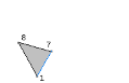
An ear of a polygon is a triangle formed by three consecutive vertices Vi0 , Vi1 , and Vi2 for which Vi1 is a
convex vertex (the interior angle at the vertex is smaller than π radians), the line segment from Vi0 to Vi2 lies completely inside the polygon, and no vertices of the polygon are contained in the triangle other than the three vertices of the triangle. In the computational geometry jargon, the line segment between Vi0 and 2 Vi2 is a diagonal of the polygon. The vertex Vi1 is called the ear tip. A triangle consists of a single ear, although you can place the ear tip at any of the three vertices. A polygon of four or more sides always has at least two nono verlapping ears [4]. This suggests a recursive approach to the triangulation. If you can locate an ear in a polygon with n ≥ 4 vertices and remove it, you have a polygon of n - 1 vertices and can repeat the process. A straightforward implementation of this will lead to an O(n3) algorithm. With some careful attention to details, the ear clipping can be done in O(n2) time. The first step is to store the polygon as a doubly linked list so that you can quickly remove ear tips. Construction of this list is an O(n) process. The second step is to iterate over the vertices and find the ears. For each vertex Vi and corresponding triangle <Vi-1,Vi,Vi+1> (indexing is modulo n, so Vn = V0 and V-1 = Vn-1), test all other vertices to see if any are inside the triangle. If none are inside, you have an ear. If at least one is inside, you do not have an ear. The actual implementation I provide tries to make this somewhat more efficient. It is sufficient to consider only reflex vertices in the triangle containment test. A reflex vertex is one for which the interior angle formed by the two edges sharing it is larger than 180 degrees. A convex vertex is one for which the interior angle is smaller than 180 degrees. The data structure for the polygon maintains four doubly linked lists simultaneously, using an array for storage rather than dynamically allocating and deallocating memory in a standard list data structure. The vertices of the polygon are stored in a cyclical list, the convex vertices are stored in a linear list, the reflex vertices are stored in a linear list, and the ear tips are stored in a cyclical list.
Once the initial lists for reflex vertices and ears are constructed, the ears are removed one at a time. If Vi is an ear that is removed, then the edge configuration at the adjacent vertices Vi-1 and Vi+1 can change. If an adjacent vertex is convex, a quick sketch will convince you that it remains convex. If an adjacent vertex is an ear, it does not necessarily remain an ear after Vi is removed. If the adjacent vertex is reflex, it is possible that it becomes convex and, possibly, an ear. Thus, after the removal of Vi, if an adjacent vertex is convex you must test if it is an ear by iterating over over the reflex vertices and testing for containment in the triangle of that vertex. There are O(n) ears. Each update of an adjacent vertex involves an earness test, a process that is O(n) per update. Thus, the total removal process is O(n2).
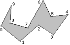
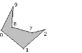
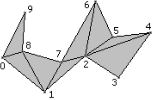
The following example, using the simple polygon of Figure 1, shows at a high level how the algorithm is structured. The initial list of convex vertices is C = {0, 1, 3, 4, 6, 9}, the initial list of reflex vertices is R = {2, 5, 7, 8}, and the initial list of ears is E = {3, 4, 6, 9}. The ear at vertex 3 is removed, so the first triangle in the triangulation is T0 = {2, 3, 4}. Figure 2 shows the reduced polygon with the new edge drawn in blue.
Figure 2. The right polygon shows the ear {2, 3, 4} removed from the left polygon.

The adjacent vertex 2 was reflex and still is. The adjacent vertex 4 was an ear and remains so. The reflex list R remains unchanged, but the edge list is now E = {4, 6, 9} (removed vertex 3).
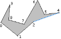
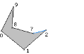
The ear at vertex 4 is removed. The next triangle in the triangulation is T1 = <2, 4, 5>. Figure 3 shows the reduced polygon with the new edge drawn in blue.
Figure 3. The right polygon shows the ear <2, 4, 5> removed from the left polygon.
The adjacent vertex 2 was reflex and still is. The adjacent vertex 5 was reflex, but is now convex. It is tested and found to be an ear. The vertex is removed from the reflex list, R = {2, 7, 8}. It is also added to the ear list, E = {5, 6, 9} (added vertex 5, removed vertex 4).
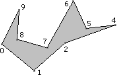
The ear at vertex 5 is removed. The next triangle in the triangulation is T2 = <2, 5, 6>. Figure 4 shows the reduced polygon with the new edge drawn in blue.
Figure 4. The right polygon shows the ear <2,5,6> removed from the left polygon.

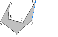
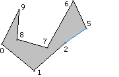
The adjacent vertex 2 was reflex, but is now convex. Although difficult to tell from the figure, the vertex 7 is inside the triangle <1, 2, 6>, so vertex 2 is not an ear. The adjacent vertex 6 was an ear and remains so.The new reflex list is R = {7,8} (removed vertex 2) and the new ear list is E = {6, 9} (removed vertex 5).The ear at vertex 6 is removed. The next triangle in the triangulation is T3 = <2, 6, 7>. Figure 5 shows the reduced polygon with the new edge drawn in blue.
Figure 5. The right polygon shows the ear <2, 6, 7> removed from the left polygon.
The adjacent vertex 2 was convex and remains so. It was not an ear, but now it becomes one. The adjacent vertex 7 was reflex and remains so. The reflect list R does not change, but the new ear list is E = {9, 2}(added vertex 2, removed vertex 6). The ear list is written this way because the new ear is added first before the old ear is removed. Before removing the old ear, it is still considered to be first in the list (well, the list is cyclical). The remove operation sets the first item to be that next value to the old ear rather than the previous value.
The ear at vertex 9 is removed. The next triangle in the triangulation is T4 = <8, 9, 0>. Figure 6 shows the reduced polygon with the new edge drawn in blue.
Figure 6. The right polygon shows the ear <8, 9, 0> removed from the left polygon.
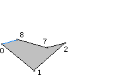
The adjacent vertex 8 was reflex, but is now convex and in fact an ear. The adjacent vertex 0 was convex and remains so. It was not an ear but has become one. The new reflex list is R = {7} and the new ear list is E = {0, 2, 8} (added 8, added 0, removed 9, the order shown is what the program produces).
The ear at vertex 0 is removed. The next triangle in the triangulation is T5 = <8, 0, 1>. Figure 7 shows the reduced polygon with the new edge drawn in blue.
Figure 7. The right polygon shows the ear <8, 0, 1> removed from the left polygon.
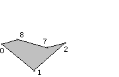
Both adjacent vertices 8 and 1 were convex and remain so. Vertex 8 remains an ear and vertex 1 remains not an ear. The reflex list remains unchanged. The new ear list is E = {2, 8} (removed vertex 0).
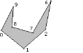
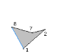
Finally, the ear at vertex 2 is removed. The next triangle in the triangulation is T6 = <1, 2, 7>. Figure 8 shows the reduced polygon with the new edge drawn in blue.
Figure 8. The right polygon shows the ear <1, 2, 7> removed from the left polygon.
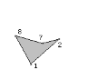
At this time there is no need to update the reflect or ear lists since we detect that only three vertices remain. The last triangle in the triangulation is T7 = <7, 8, 1>. The full triangulation is show in Figure 9.
Figure 9. The full triangulation of the original polygon.
3 Polygons with a Hole
The ear-clipping algorithm may also be applied to polygons with holes. First, consider a polygon with one hole, as shown in Figure 10. It consists of an outer polygon and an inner polygon. The ordering of the outer vertices and the inner vertices must be opposite. If the outer vertices are counterclockwise ordered, then the inner vertices must be clockwise ordered.
Figure 10. A polygon with a hole.
The blue vertices are mutually visible. We can convert this to the topology of a simple polygon by introducing two coincident edges connecting the blue-colored vertices. Figure 11 shows the two new edges, one drawn in blue and one drawn next to it in red. The edges are coincident; drawing them as shown just illustrates there are two edges.
Figure 11. The polygon hole is removed by introducing two new edges that “cut” open the polygon.
4 Finding Mutually Visible Vertices
Visually, we can see in Figure 10 that vertices V11 and V16 are mutually visible. In fact, there are many more such pairs, one vertex from the outer polygon and one vertex from the inner polygon. We need an algorithm that will find a pair of mutually visible vertices.
One such algorithm is the following. Search the vertices of the inner polygon to find the one with maximum x-value. In Figure 10, this is V16. Imagine an observer standing at this this vertex, looking in the positive x-direction. He will see (1) an interior point of an edge or (2) a vertex, an interior point of an edge being the most probable candidate. If a vertex is visible, then we have a mutually visible pair.
Consider, though, that the closest visible point in the positive x-direction is an interior edge point, as illustrated in Figure 12.
Figure 12. The closest visible point is an interior edge point.
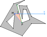
Let M be the origin of the ray (in the example, V16). The ray M + t(1, 0) is shown in blue. The closest visible point is shown in red, call this point I. The edge on which the closest point occurs is drawn in green. The endpoint of the edge that has maximum x-value is labeled P. The point P is the candidate for mutual visibility with M. The line segment connecting them is drawn in purple. The triangle <M, I, P> is drawn with an orange interior.
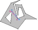
In 12, P is indeed visible to M. Generally, it is possible that other edges of the outer polygon cross the line segment <M, P>, in which case P is not visible to M. Figure 13 shows such a situation.
Figure 13. A case where P is not visible to M.
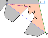
The gray color denotes the region between the outer and inner polygons. The orange region is also part of the interior. In 12, the entire interior of triangle <M, I, P> is part of the outer-inner interior. In 13, the outer polygon cuts into the triangle, so only a subset of the triangle interior is part of the outer-inner interior.
Four vertices of the outer polygon occur inside triangle <M, I, P>. Generally, if vertices occur inside this triangle, at least one must be reflex. And of all such reflex vertices, one must be visible to M. In Figure 13, three reflex vertices of the outer polygon occur inside the triangle. They are labeled A, B, and C. The reflex vertex A is visible to M, because it minimizes the angle θ between (1, 0) and the line segments <M, R>, where R is any reflex vertex.
The algorithm is summarized as:
1.Search the inner polygon for vertex M of maximum x-value.
2. Intersect the ray M + t (1, 0) with all directed edges <Vi, Vi+1> of the outer polygon for which M is to the left of the line containing the edge (M is inside the outer polygon). Let I be the closest visible point to M on this ray.
3. If I is a vertex of the outer polygon, then M and I are mutually visible and the algorithm terminates.
4. Otherwise, I is an interior point of the edge <Vi, Vi+1>. Select P to be the endpoint of maximum x-value for this edge.
5. Search the reflex vertices of the outer polygon (not including P if it happens to be reflex). If all of these vertices are strictly outside triangle <M, I, P>, then M and P are mutually visible and the algorithm terminates.
6. Otherwise, at least one reflex vertex lies in <M, I, P>. Search for the reflex R that minimizes the angle between (1, 0) and the line segment <M, R>. Then M and R are mutually visible and the algorithm terminates. It is possible in this step that there are multiple reflex vertices that minimize the angle, in which case all of them lie on a ray with M as the origin. Choose the reflex vertex on this ray that is closest to M.
5 Polygons with Multiple Holes
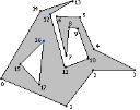
A polygon may have multiple holes (inner polygons). The assumptions are that they are all strictly contained by the outer polygon and none of them overlap. Figure 14 shows such a polygon.
Figure 14. An outer polygon with two inner polygons.
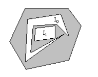
The figure makes it clear that none of the vertices of inner polygon I1 are visible to the outer polygon vertices. However, some vertices of inner polygon I0 are visible to outer polygon vertices. Thus, we may use the previously mentioned algorithm to combine the outer polygon and I0 into a simple polygon. This polygon becomes the new outer polygon and I1 is combined with it to form yet another simple polygon. This final polygon is triangulated by ear clipping.
Given multiple inner polygons, the one containing the vertex of maximum x-value of all inner polygon vertices is the one chosen to combine with the outer polygon. The process is then repeated with the new outer polygon and the remaining inner polygons.
6 Hierarchies of Polygons
The inner polygons themselves can contain outer polygons with holes, thus leading to trees of nested polygons. The root of the tree corresponds to the outermost outer polygon. The children of the root are the inner polygons contained in this outer polygon. Each grandchild (if any) is a subtree whose root corresponds to an outer polygon that is strictly contained in the parent inner polygon and whose own children are inner polygons. A tree of polygons may be processed using a breadth-first traversal.
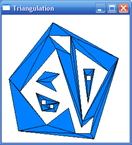
Figure 15 shows a tree of nested polygons that has been triangulated using ear clipping.
Figure 15. A tree of nested polygons (see SampleFoundation/Triangulation).
The tree and its nodes are abstractly shown here:
outer0
    inner0
    inner1
        outer1
        outer2
            inner3
            inner4
        outer3
            inner5
    inner2
The pseudocode for processing the tree is
struct PolygonTree
{
    Polygon p;
    array<PolygonTree> children;
};
array<Triangle> triangles;
PolygonTree tree = <some tree of polygons>;
queue<PolygonTree> Q;
Q.insertRear(tree);
while (not Q.empty()) do
{
    PolygonTree outerNode = Q.removeFront();
    numChildren = outerNode.children.quantity();
    if (numChildren == 0)
    {
        // The outer polygon is a simple polygon with no nested inner
        // polygons.
        triangles.append(GetEarClipTriangles(outerNode.p));
    }
    else
    {
        // The outer polygon contains inner polygons.
        for (i = 0; i < numChildren; i++)
        {
            PolygonTree innerNode = outerNode.children[i];
            array<Polygon> innerPolygons;
            numGrandchildren = innerNode.children.quantity();
            for (j = 0; j < numGrandchildren; j++)
            {
                innerPolygons.append(innerNode.p);
                Q.insertFront(innerNode.children[j]);
            }
        }
        Polygon combined = MakeSimple(outerNode.p,innerPolygons);
        triangles.append(GetEarClipTriangles(combined));
    }
}
The function MakeSimple encapsulates the algorithm described previously for finding two mutually visible vertices for an outer and an inner polygon, and then duplicates them and inserts two new edges to produce a simple polygon. The process is repeated for each inner polygon.
The final triangulation is actually postprocessed so that the indices for the duplicated vertices are replaced by indices for the original vertices. This is slightly tricky in that duplicated vertices can themselves be duplicated-you need to follow the chains of indices back to their original values.
References
[1] B. Chazelle and J. Incerpi, Triangulation and shape complexity, ACM Trans. on Graphics, vol. 3, pp. 135-152, 1984.
[2] B. Chazelle, Triangulating a simple polygon in linear time, Discrete Comput. Geom., vol. 6, pp. 485-524, 1991.
[3] A. Fournier and D.Y. Montuno, Triangulating simple polygons and equivalent problems, ACM Trans.on Graphics, vol. 3, pp. 153-174, 1984.
[4] G.H. Meisters, Polygons have ears, Amer. Math. Monthly, vol. 82, pp. 648-651, 1975.
[5] R. Seidel, A simple and fast incremental randomized algorithm for computing trapezoidal decompositions and for triangulating polygons, Computational Geometry: Theory and Applications, vol. 1, no.1, pp. 51-64, 1991.
