cp11_13_Object Orientation And Graphical User Interfaces(安装install trait)

First, solve the problem. Then, write the code. — Jon Johnson

It might be helpful to have (class/object) private attributes. These are generally indicated by one or two leading underscores, as the following class definition illustrates:

def mulplication(self):
    return self.a * self.b
class ExampleSeven(object):
    def __init__(self, a,b):
        self.a = a
        self.b =b
        self.__sum=a+b #two leading undersores can be accessed by c._ExampleSeven__sum
    multiplication = mulplication
    def addition(self):
        return self.__sum

c=ExampleSeven(10,15)
c.addition()

c._ExampleSeven__sum

c.a += 10
c.a

c.addition()

#25 #This is due to the fact that the private attribute self.__sum is not updated:

c.multiplication() #multiplication is referecing the global method

class sorted_list(object):
    def __init__(self, elements):
        self.elements = sorted(elements) # sorted list object
    def __iter__(self):
        self.position = -1
        return self
    def __next__(self):
        if self.position == len(self.elements) - 1:
            raise StopIteration
        self.position += 1
        return self.elements[self.position]

name_list = ['Sandra','Lilli', 'Guido', 'Zorro', 'Henry']
sorted_name_list = sorted_list(name_list)
for name in sorted_name_list:
    print(name)

type(sorted_name_list)

Simple Short Rate Class

(note:discounting since the future value of money is not the same as today's value, and usually the future cash flow is worthless compared to today)

One of the most fundamental concepts in finance is discounting折现. Since it is so fundamental, it might justify the definition of a discounting class. In a constant short rate world with continuous discounting, the factor to discount a future cash flow due at date t >0 to the present t = 0 is defined by .

Consider first the following function definition, which returns the discount factor for a given future date and a value for the constant short rate. Note that a NumPy universal function is used in the function definition for the exponential function to allow for vectorization:

import numpy as np

def discount_factor(r,t):
    #returns the discount factor for a given future date(t) and a value for the constant short rate(r)
    df = np.exp(-r*t)
    return df

illustrates how the discount factors behave for different values for the constant short rate over five years. The factors for t = 0 are all equal to 1; i.e., “no discounting” of today’s cash flows. However, given a short rate of 10% and a cash flow due in five years, the cash flow would be discounted to a value slightly above 0.6 per currency unit (i.e., to 60%). We generate the plot as follows:

import matplotlib.pyplot as plt
%matplotlib inline

t = np.linspace(0,5)
for r in [0.01, 0.05, 0.1]:
    plt.plot(t, discount_factor(r,t), label='r=%4.2f' % r , lw=1.5)
plt.xlabel('years')
plt.ylabel('discount factor')
plt.grid(True)
plt.legend(loc='best') #loc=0: left bottom

Explain：If the short-term interest rate is smaller, the fluctuation of the discount factor in the future is smaller; otherwise, if the higer the short-term interest rate, the greater the fluctuation of the discount factor in the future(It becomes smaller); In other words, if the short-term rate is higher, the future money will be less valuable since the future money will be discounted lesser (than today).

For comparison, now let us look at the class-based implementation approach. We call it short_rate since this is the central entity/object and the derivation of discount factors is accomplished via a method call

class Short_Rate(object):
    #returns discount factors(Array) for given list/array of dates/times (as year fractions)
    def __init__(self, name, rate):
        self.name = name #string, name of the object
        self.rate = rate #float positive, constant short rate
    def get_discount_factors(self, time_list):
        time_list = np.array(time_list)
        return np.exp(-self.rate*time_list)

shortRate = Short_Rate('r', 0.05)
shortRate.name, shortRate.rate

To get discount factors from the new object, a time list with year fractions is needed:

time_list = [0.0, 0.5, 1.0, 1.25, 1.75, 2.0] # in year fractions
shortRate.get_discount_factors(time_list)

Using this object, it is quite simple to generate a plot as before (see previous figure). The major difference is that we first update the attribute rate and then provide the time list t to the method get_discount_factors:

t = np.linspace(0,5) #t = np.linspace(0,5,n)# 0, 5/(n-1),5/(n-1) *2..., 5 #total number is equal to n
for r in [0.025, 0.05, 0.1, 0.15]:
    shortRate.rate = r
    plt.plot(t, shortRate.get_discount_factors(t), 
             label='r=%4.2f'%shortRate.rate, lw=1.5)
    
plt.xlabel('years')
plt.ylabel('discount factor')
plt.title('Discount factors for different short rates over five years')
plt.grid(True)
plt.legend(loc=0)

Generally, discount factors are “only” a means to an end 折现闲子"只是"达到某种目的的手. For example, you might want to use them to discount future cash flows. With our short rate object, this is an easy exercise when we have the cash flows and the dates/times of their occurrence available. Consider the following cash flow example, where there is a negative cash flow today and positive cash flows after one year and two years, respectively. This could be the cash flow profile of an investment opportunity:

shortRate.rate = 0.05
cash_flows = np.array([-100, 50, 75])
time_list = [0.0, 1.0, 2.0]

disc_facts = shortRate.get_discount_factors(time_list)
disc_facts

#（First, we should calculate the discount factors, eg ）

# present values
disc_facts * cash_flows

#(Second, we should calculate the present value(现值）#cash flow * e^(-rt),eg

A typical decision rule in investment theory says that a decision maker should invest into a project whenever the net present value (NPV), given a certain (short) rate representing the opportunity costs of the investment投资的机
会成本, is positive. In our case, the NPV is simply the sum of the single present values:

# net present value
np.sum(disc_facts*cash_flows)

Obviously, for a short rate of 5% the investment should be made(Explain: If we initially invest $100, the actually return rate is 15.424277577732667% higher then the investment). What about a rate of 15%(Explain: the higher short-term rate, the lower the factor to discount that will reduced the value of future cash flow)? Then the NPV becomes negative, and the investment should not be made:

shortRate.rate = 0.15
np.sum(shortRate.get_discount_factors(time_list) * cash_flows)

#Explain: the future return is less than the initial investment.((1-1.4032)*100) <100, the investment should not be made

Cash Flow Series Class

With the experience gained through the previous example, the definition of another class to model a cash flow series should be straightforward. This class should provide methods to give back a list/array of present values and also the net present value(净现值) for a given cash flow series — i.e., cash flow values and dates/times:

class Short_Rate(object):
    #returns discount factors(Array) for given list/array of dates/times (as year fractions)
    def __init__(self, name, rate):
        self.name = name #string, name of the object
        self.rate = rate #float positive, constant short rate
    def get_discount_factors(self, time_list):
        time_list = np.array(time_list)
        return np.exp(-self.rate*time_list)
    
class Cash_Flow_Series(object): #Class to model a cash flow series
    def __init__(self, name, time_list, cash_flows, Short_Rate):
        #short_rate: instance of short_rate class #short rate object used for discounting
        self.name = name
        self.time_list = time_list
        self.cash_flows = cash_flows
        self.Short_Rate = Short_Rate
        
    def present_value_list(self): #returns an array with present νalues
        df = self.Short_Rate.get_discount_factors(self.time_list)
        return np.array(self.cash_flows) * df
    
    def net_present_value(self):
        return np.sum(self.present_value_list())

#shortRate = short_rate('r', 0.05) #time_list = [0.0, 1.0, 2.0]
shortRate.rate=0.05
cashFlowSeries=Cash_Flow_Series('cfs', time_list, cash_flows, shortRate)
cashFlowSeries.cash_flows

cashFlowSeries.time_list

We can now compare the present values and the NPV with the results from before. Fortunately, we get the same results:

cashFlowSeries.present_value_list()

cashFlowSeries.net_present_value()

There is further potential to generalize the steps of the previous example. One option is to define a new class that provides a method for calculating the NPV for different short rates — i.e., a sensitivity analysis. We use, of course, the cash_flow_series class to inherit from:

import numpy as np

#shortRate = Short_Rate('r', 0.0) #global variable

class Short_Rate(object):
#returns discount factors(Array) for given list/array of dates/times (as year fractions)
def __init__(self, name, rate):
self.name = name #string, name of the object
self.rate = rate #float positive, constant short rate
def get_discount_factors(self, time_list):
time_list = np.array(time_list)
return np.exp(-self.rate*time_list)

class Cash_Flow_Series(object): #Class to model a cash flow series
def __init__(self, name, time_list, cash_flows, Short_Rate):
#short_rate: instance of short_rate class #short rate object used for discounting
self.name = name
self.time_list = time_list
self.cash_flows = cash_flows
self.Short_Rate = Short_Rate

def present_value_list(self): #returns an array with present νalues
df = self.Short_Rate.get_discount_factors(self.time_list)
return np.array(self.cash_flows) * df

def net_present_value(self):
return np.sum(self.present_value_list())

class CashFlowSeries_Sensitivity(Cash_Flow_Series):
#provides a method for calculating the NPV for different short rates
def npv_sensitivity(self, short_rateList):
npvs = []
for rate in short_rateList:
#shortRate.rate = rate #shortRate is a global variable #another way
self.Short_Rate.rate = rate #Short_Rate inherit from class cash_flow_series
npvs.append(self.net_present_value()) #net_present_value() inherit from class Cash_Flow_Series
return np.array(npvs)

time_list = [0.0, 1.0, 2.0] # in year fractions
cash_flows = np.array([-100, 50, 75])
shortRate = Short_Rate('r', 0.05)
#shortRate.rate = 0.05
cashflowseries_sens = CashFlowSeries_Sensitivity('cfs', time_list, cash_flows, shortRate)

For example, defining a list containing different short rates, we can easily compare the resulting NPVs:

short_rateList = [0.01, 0.025, 0.05, 0.075, 0.1, 0.125, 0.15, 0.2]
npvs = cashflowseries_sens.npv_sensitivity(short_rateList)
npvs

Explain：The lower short-term interest rate, the higher the NPV, indicating the future is a posive cash flow(the value of future cash flow is high), because the lower the interest rate, the higher the discount factor.

shows the result graphically. The thicker horizontal line (at 0) shows the cutoff point分界点 between a profitable investment and one that should be dismissed given the respective (short) rate:

import matplotlib.pyplot as plt

plt.plot(short_rateList, npvs, 'b')
plt.plot(short_rateList, npvs, 'ro')
plt.plot( (0, max(short_rateList)), (0,0), 'r', lw=2 )
plt.grid(True)
plt.xlabel('short rate')
plt.ylabel('net present value')
plt.title('Net present values of cash flow list for different short rates')

Explain: The thicker horizontal line (at 0) shows the cutoff point分界点 between a profitable investment and one that should be dismissed given the respective (short) rate

Graphical User Interfaces

To build the GUIs we use the traits library, documentation of which you can find at http://code.enthought.com/projects/traits/docs/html/index.html. traits is generally used for rapid GUI building on top of existing classes and only seldom for more complex applications. In what follows, we will reimplement the two example classes from before, taking into account that we want to use a GUI for interacting with instances of the respective classes.

Source Code in github: https://github.com/enthought/traitsui

https://pypi.org/project/traits/

https://anaconda.org/anaconda/traits

#First I install trait by using Anaconda Navigator 1.9.7 OR Anaconda 2019.03 python 2.7

For the definition of our new short_rate class, we use the HasTraits class to inherit from. Also note in the following class definition that traits has its own data types, which are generally closely intertwined with visual elements of a GUI — to put it differently, traits knows which graphical elements (e.g., for a text field) to use to build a GUI (semi)automatically:

import numpy as np
import traits.api as trapi

class Short_Rate(trapi.HasTraits): #class Short_Rate inherits from HasTraits
    name = trapi.Str #1 cell
    rate = trapi.Float # 1 cell
    time_list = trapi.Array(dtype=np.float, shape=(5,)) #5 rows & 1 column cells
    
    def get_discount_factors(self):
        return np.exp(-self.rate * self.time_list)
    
sr = Short_Rate()

sr.configure_traits() #via a call of the method configure_traits (inherited from HasTraits) a GUI is
#automatically generated, and we can use this GUI to input values for the attributes of the
#new object sr:

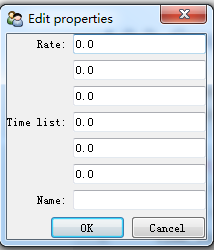
shows such a simple GUI, which in this case is still empty. （Note that the middle five fields all belong to “Time list” — this layout is generated by default.）Then enter your value

Then click OK button

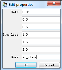
In effect, this gives the same results as the following lines of code:

sr.name = ‘sr_class’
sr.rate = 0.05
sr.time_list = [0.0, 0.5, 1.0, 1.5, 2.0]

Updating of Values

So far, the new short_rate class using traits allows us to input data for initializing attributes of an instance of the class. However, a GUI usually is also used to present results. You would generally want to avoid providing input data via a GUI and then making the user access the results via interactive scripting. To this end, we need another sublibrary, traitsui.api:

import traits.api as trapi
import traitsui.api as trui

class Short_Rate(trapi.HasTraits):
    name = trapi.Str #can't not define self.name
    rate = trapi.Float #can't not define self.rate
    time_list = trapi.Array(dtype=np.float, shape=(1,5))
    disc_factor_list = trapi.Array(dtype=np.float, shape=(1,5))
    
    update = trapi.Button
    def _update_fired(self):
        self.disc_factor_list = np.exp(-self.rate * self.time_list)
    
    v = trui.View(trui.Group(trui.Item(name='name'),
                             trui.Item(name='rate'),
                             trui.Item(name='time_list', label='Insert Time List Here'),
                             trui.Item(name='update', show_label=False),
                             trui.Item(name='disc_factor_list', label='Press Update for Factors'),
                             show_border=True,#show margin
                             label='Calculate Discount Factors'
                            ),
                    buttons = [trui.OKButton, trui.CancelButton],
                    resizable=True
                 )

sr = Short_Rate()
sr.configure_traits()

Then enter the value

sr.name = ‘sr_class’
sr.rate = 0.05
sr.time_list = np.array(([0.0, 0.5, 1.0, 1.5, 2.0],), dtype=np.float32)

then click Update button,

sr._update_fired()

finally click OK button

sr.disc_factor_list

Cash Flow Series Class with GUI

The last example in this section is about the cash_flow_series class. In principle, we have seen in the previous example the basic workings of traits when it comes to presenting results within a GUI window. Here, we only want to add some twists to the
story: for example, a slider to easily change the value for the short rate. In the class definition that follows, this is accomplished by using the Range function, where we provide a minimum, a maximum, and a default value. There are also more output fields to account for the calculation of the present values and the net present value:

import traits.api as trapi
import traitsui.api as trui

class Cash_Flow_Series(trapi.HasTraits):
    name = trapi.Str
                            #min  max  default
    short_rate = trapi.Range(0.0, 0.5, 0.05)
    time_list = trapi.Array(dtype=np.float, shape=(1,6))
    cash_flow_list = trapi.Array(dtype=np.float, shape=(1,6))
    disc_factor_list = trapi.Array(dtype=np.float, shape=(1,6))
    present_value_list = trapi.Array(dtype=np.float, shape=(1,6))
    net_present_value = trapi.Float
    update = trapi.Button
    
    def _update_fired(self):
        self.disc_factor_list = np.round( np.exp(-self.short_rate * self.time_list),6)
        self.present_value_list = np.round( self.disc_factor_list * self.cash_flow_list,6)
        self.net_present_value = np.round( np.sum(self.present_value_list),6)
        
    v = trui.View(trui.Group(trui.Item(name='name'),
                             trui.Item(name='short_rate'),
                             trui.Item(name='time_list', label='Time List'),
                             trui.Item(name='cash_flow_list', label='Cash Flows'),
                             trui.Item('update', show_label=False),
                             trui.Item(name='disc_factor_list', label='Discount Factors'),
                             trui.Item(name='present_value_list', label='Present_Values'),
                             trui.Item(name='net_present_value', label='Net Present Value'),
                             show_border =True, 
                             label='Calculate Present Values'
                            ),
                  buttons = [trui.OKButton, trui.CancelButton],
                  resizable=True
                 )
    
cfs = Cash_Flow_Series()
cfs.configure_traits()
    
cfs = Cash_Flow_Series()
cfs.configure_traits()

Input: The GUI allows for inputting data to initialize all object attributes.
Logic: There is application logic that calculates discount factors, present values, and an NPV.
Output: The GUI presents the results of applying the logic to the input data.

Then enter values