机器学习——推荐系统

（一）SVD原理分析

人能够对一些事物的重要特征做抽象提取，奇异值分解（Singular Value Decomposition，SVD正是机器抽象提取一些事物重要特征的方法。利用SVD， 可使用小得多的数据集来表示原始数据集，这样会去除噪声数据和冗余信息。

最早的SVD应用之一是信息检索。将利用SVD的方法称为隐性语义索引（Latent Semantic Indexing，LSI）或隐性语义分析（Latent Semantic Analysis，LSA）。

SVD的另一个应用是推荐系统。简单版本的推荐系统能计算项或人之间的相似度。更先进的方法则先利用SVD从数据中构建一个主题空间，然后再在该空间下计算其相似度。

矩阵分解
在很多情况下，数据中的一小段携带了数据集中的大部分信息，而其他信息要么是噪声，要么就是毫不相关的信息。矩阵分解可将原始矩阵表示成新的易于处理的形式，新形式是两个或多个矩阵的乘积。

不同的矩阵分解技术具有不同的性质，其中有些更适合于某个应用，有些则更适合于其他应用。最常见的一种矩阵分解技术就是SVD。SVD将原始的数据集矩阵Data分解成三个矩阵 $U$、 $Σ$、 $V^{T}$。如果原始矩阵Data是m行n列，则有如下等式：
$Data_{m\times n}=U_{m\times m}\Sigma _{m\times n}V_{n\times n}^{T}$

上述分解中会构建出一个矩阵 $Σ$，该矩阵只有对角元素，其他元素均为0。另一个惯例就是， $Σ$的对角元素是从大到小排列的。这些对角元素称为奇异值（Singular Value），它们对应了原始数据集矩阵Data的奇异值。奇异值和特征值时有关系的。这里的奇异值就是矩阵 $Data∗Data^{T}$特征值的平方根。

矩阵 $Σ$只有从大到小排列的对角元素。在科学和工程中，一致存在这样一个普遍事实：在某个奇异值的数目（r个）之后，其他的奇异值都置为0。这就意味着数据集中仅有r个重要特征，而其余特征则都是噪声或冗余特征。

利用Python实现SVD
NumPy由一个称为linalg的线性代数工具箱，利用此工具箱可实现如下矩阵的SVD处理：

from numpy import *
U,Sigma,VT=linalg.svd([[1,1],[7,7]])
U

array([[-0.14142136, -0.98994949],
[-0.98994949, 0.14142136]])

Sigma

array([1.00000000e+01, 2.82797782e-16])

VT

array([[-0.70710678, -0.70710678],
[ 0.70710678, -0.70710678]])

接下来在一个更大的数据集上进行更多的分解:

def loadExData() :
    return [[1, 1, 1, 0, 0],
            [2, 2, 2, 0, 0],
            [1, 1, 1, 0, 0],
            [5, 5, 5, 0, 0],
            [1, 1, 0, 2, 2],
            [0, 0, 0, 3, 3],
            [0, 0, 0, 1, 1]]
import svdRec as svdRec
Data=svdRec.loadExData()
U,Sigma,VT=linalg.svd(Data)
Sigma

array([9.72140007e+00, 5.29397912e+00, 6.84226362e-01, 4.11502614e-16,
1.36030206e-16])

前三个数据比其他的值大很多，后两个值在不同机器上结果可能会稍有差异，但数量级差不多。于是，我们可将后两个值去掉。原始数据集可用如下结果来近似：
$Data_{m\times n}=U_{m\times 3}\Sigma _{3\times 3}V_{3\times n}^{T}$

重构原始矩阵，首先构建一个3x3的矩阵Sig3：

Sig3=mat([[Sigma[0], 0, 0],[0, Sigma[1], 0],[0, 0, Sigma[2]]])

由于Sig3仅为3x3的矩阵，因而只需使用矩阵U的前3列和VT的前三行。为了在Python中实现这一点，输入如下命令：

U[:,:3]*Sig3*VT[:3,:]

matrix([[ 1.00000000e+00, 1.00000000e+00, 1.00000000e+00,
7.75989921e-16, 7.71587483e-16],
[ 2.00000000e+00, 2.00000000e+00, 2.00000000e+00,
3.00514919e-16, 2.77832253e-16],
[ 1.00000000e+00, 1.00000000e+00, 1.00000000e+00,
2.18975112e-16, 2.07633779e-16],
[ 5.00000000e+00, 5.00000000e+00, 5.00000000e+00,
3.00675663e-17, -1.28697294e-17],
[ 1.00000000e+00, 1.00000000e+00, -5.48397422e-16,
2.00000000e+00, 2.00000000e+00],
[ 3.21319929e-16, 4.43562065e-16, -3.48967188e-16,
3.00000000e+00, 3.00000000e+00],
[ 9.71445147e-17, 1.45716772e-16, -1.52655666e-16,
1.00000000e+00, 1.00000000e+00]])

（二）餐馆菜肴推荐系统

有很多方法可实现推荐功能，这里使用一种称为协同过滤（collaborative filtering）的方法。协同过滤是通过将用户和其他用户的数据进行对比来实现推荐的。

当知道两个用户或两个物品之间的相似度，就可利用已有的数据来预测未知的用户喜好。

下面计算一下手撕猪肉和烤牛肉之间的相似度。一开始使用欧氏距离来计算。

$\sqrt{(4-4)^{2}+(3-3)^{2}+(2-1)^{2}}=1$

而手撕猪肉和鳗鱼饭的欧式距离为：

$\sqrt{(4-2)^{2}+(3-5)^{2}+(2-2)^{2}}=2.83$

在该数据中，由于手撕猪肉和烤牛肉的距离小于手撕猪肉和鳗鱼饭的距离。因此手撕猪肉与烤牛肉比鳗鱼饭更为相似。我们希望，相似度值在0到1之间变化，并且物品对越相似，它们的相似度值也就越大。
$相似度=1/(1+距离)$当距离为0时，相似度为1.0。如果距离真的非常大时，相似度也就趋近于0。

第二种计算距离的方法是皮尔逊相关系数（Pearson correlation）。在度量回归方程的精度时曾经用到过这个量，它度量的是两个向量之间的相似度。该方法相对于欧式距离的一个优势在于，它对用户评级的量级并不敏感。比如，某个狂躁者对所有物品的评分都是5分，而另一个忧郁者对所有物品的评分都是1分，皮尔逊相关系数会认为这两个向量时相等的。在NumPy中，皮尔逊相关系数的计算是由函数corrcoef()进行的，后面很快就会用到它了。皮尔逊相关系数取值范围从-1到+1，可通过0.5+0.5*corrcoef()这个函数计算，并且把其取值范围归一化到0到1之间。

另一个常用的距离计算方法是余弦相似度（cosine similarity），其计算的是两个夹角的余弦值。如果夹角为90度，则相似度为0；如果两个向量的方向相同，则相似度为1.0。同皮尔逊相关系数一样，余弦相似度的取值范围也在-1到+1之间，因此也需将它归一化到0到1之间。计算余弦相似度，采用的两个向量AA和BB夹角的余弦相似度的定义如下：
$cos\theta =\frac{A\cdot B}{||A||||B||}$

其中，表示向量A、B的2范数，还可以定义向量的任一范数，但是如果不指定范数阶数，则都假设为2范数。向量[4, 2, 2]的2范数为：

$\sqrt{(4)^{2}+(2)^{2}+(2)^{2}}$

将上述各种相似度的计算方法写成Python中的函数。

from numpy import *
from numpy import linalg as la
# inA和inB都是列向量
def ecludSim(inA, inB) :
    return 1.0/(1.0 + la.norm(inA - inB))

def pearsSim(inA, inB) :
    # 检查是否存在三个或更多的点，若不存在，则返回1.0，这是因为此时两个向量完全相关
    if len(inA) < 3 : return 1.0
    return 0.5+0.5*corrcoef(inA, inB, rowvar = 0)[0][1]

def cosSim(inA, inB) :
    num = float(inA.T*inB)
    denom = la.norm(inA)*la.norm(inB)
    return 0.5+0.5*(num/denom)

import ml.svdRec as svdRec
from numpy import *
myMat = mat(svdRec.loadExData())
# 欧氏距离
svdRec.ecludSim(myMat[:,0], myMat[:,4])
0.13367660240019172
svdRec.ecludSim(myMat[:,0], myMat[:,0])
1.0

# 余弦相似度
svdRec.cosSim(myMat[:,0], myMat[:,4])
0.54724555912615336
svdRec.cosSim(myMat[:,0], myMat[:,0])
0.99999999999999989

# 皮尔逊相关系数
svdRec.pearsSim(myMat[:,0], myMat[:,4])
0.23768619407595826
svdRec.pearsSim(myMat[:,0], myMat[:,0])
1.0

上面计算了两个餐馆菜肴之间的距离，这称为基于物品（item-based）的相似度。计算用户距离的方法则称为基于用户（user-based）的相似度。行与行之间比较的是基于用户的相似度，列与列之间比较的是基于物品的相似度。使用哪种相似度取决于用户或物品的数目。基于物品相似度计算的时间会随着物品数量的增加而增加，基于用户的相似度计算的时间则会随着用户数量的增加而增加。如果用户的数目很多，那么我们可能倾向于使用基于物品相似度的计算方法。

推荐系统的工作过程是：给定一个用户，系统会为此用户返回N个最好的推荐菜。为了实现这一点，则需要做到：

1. 寻找用户没有评级的菜肴，即在用户-物品矩阵中的0值；
2. 在用户没有评级的所有物品中，对每个物品预计一个可能的评级分数。这就是说，我们认为用户可能对物品的打分（这就是相似度计算的初衷）；
3. 对这些物品的评分从高到底进行排序，返回前N个物品。

基于物品相似度的推荐引擎代码如下：

# 用来计算在给定相似度计算方法的条件下，用户对物品的估计评分值
# 参数：数据矩阵、用户编号、物品编号、相似度计算方法，矩阵采用图1和图2的形式
# 即行对应用户、列对应物品
def standEst(dataMat, user, simMeas, item) :
    # 首先得到数据集中的物品数目
    n = shape(dataMat)[1]
    # 对两个用于计算估计评分值的变量进行初始化
    simTotal = 0.0; ratSimTotal = 0.0
    # 遍历行中的每个物品
    for j in range(n) :
        userRating = dataMat[user,j]
        # 如果某个物品评分值为0，意味着用户没有对该物品评分，跳过
        if userRating == 0 : continue
        # 寻找两个用户都评级的物品，变量overLap给出的是两个物品当中已经被评分的那个元素
        overLap = nonzero(logical_and(dataMat[:, item].A>0, dataMat[:, j].A>0))[0]
        # 若两者没有任何重合元素，则相似度为0且中止本次循环
        if len(overLap) == 0 : similarity = 0
        # 如果存在重合的物品，则基于这些重合物品计算相似度
        else : similarity = simMeas(dataMat[overLap, item], dataMat[overLap, j])
        # print 'the %d and %d similarity is : %f' % (item, j, similarity)
        # 随后相似度不断累加
        simTotal += similarity
        ratSimTotal += similarity * userRating
    if simTotal == 0 : return 0
    # 通过除以所有的评分总和，对上述相似度评分的乘积进行归一化。这使得评分值在0-5之间，
    # 而这些评分值则用于对预测值进行排序
    else : return ratSimTotal/simTotal

# 推荐引擎，会调用standEst()函数，产生最高的N个推荐结果。
# simMeas：相似度计算方法
# estMethod：估计方法
def recommend(dataMat, user, N=3, simMeas=cosSim, estMethod=standEst) :
    # 寻找未评级的物品，对给定用户建立一个未评分的物品列表
    unratedItems = nonzero(dataMat[user, :].A==0)[1]
    # 如果不存在未评分物品，退出函数，否则在所有未评分物品上进行循环
    if len(unratedItems) == 0 : return 'you rated everything'
    itemScores = []
    for item in unratedItems :
        # 对于每个未评分物品，通过调用standEst()来产生该物品的预测评分。
        estimatedScore = estMethod(dataMat, user, simMeas, item)
        # 该物品的编号和估计得分值会放在一个元素列表itemScores
        itemScores.append((item, estimatedScore))
    # 寻找前N个未评级物品
    return  sorted(itemScores, key=lambda jj : jj[1], reverse=True)[:N] 

import ml.svdRec as svdRec
from numpy import *
#调入原始矩阵
myMat=mat(svdRec.loadExData())
#该矩阵对于展示SVD的作用非常好，但是它本身不是十分有趣，因此我们要对其中的一些值进行更改
myMat[0,1]=myMat[0,0]=myMat[1,0]=myMat[2,0]=4
myMat[3,3]=2
#得到矩阵如下
myMat
matrix([[4, 4, 1, 0, 0],
        [4, 2, 2, 0, 0],
        [4, 1, 1, 0, 0],
        [5, 5, 5, 2, 0],
        [1, 1, 0, 2, 2],
        [0, 0, 0, 3, 3],
        [0, 0, 0, 1, 1]])
#尝试默认推荐
svdRec.recommend(myMat,2)
#表明用户2对物品4的预测评分值为2.5，对物品3的预测评分值为1.9
[(4, 2.5), (3, 1.9703483892927431)]
#利用其它相似度计算方法来计算推荐
svdRec.recommend(myMat,2,simMeas=svdRec.ecludSim)
[(4, 2.5), (3, 1.9866572968729499)]
svdRec.recommend(myMat,2,simMeas=svdRec.pearsSim)
[(4, 2.5), (3, 2.0)]

利用SVD提高推荐的效果
实际的数据集会比用于展示recommend()函数功能的myMat矩阵稀疏得多。

def loadExData2():
    return[[0, 0, 0, 0, 0, 4, 0, 0, 0, 0, 5],
           [0, 0, 0, 3, 0, 4, 0, 0, 0, 0, 3],
           [0, 0, 0, 0, 4, 0, 0, 1, 0, 4, 0],
           [3, 3, 4, 0, 0, 0, 0, 2, 2, 0, 0],
           [5, 4, 5, 0, 0, 0, 0, 5, 5, 0, 0],
           [0, 0, 0, 0, 5, 0, 1, 0, 0, 5, 0],
           [4, 3, 4, 0, 0, 0, 0, 5, 5, 0, 1],
           [0, 0, 0, 4, 0, 4, 0, 0, 0, 0, 4],
           [0, 0, 0, 2, 0, 2, 5, 0, 0, 1, 2],
           [0, 0, 0, 0, 5, 0, 0, 0, 0, 4, 0],
           [1, 0, 0, 0, 0, 0, 0, 1, 2, 0, 0]]

接下来计算该矩阵的SVD来了解其到底需要多少维特征。

from numpy import linalg as la
from numpy import *
U,Sigma,VT=la.svd(mat(svdRec.loadExData2()))
Sigma

array([ 15.77075346, 11.40670395, 11.03044558, 4.84639758,
3.09292055, 2.58097379, 1.00413543, 0.72817072,
0.43800353, 0.22082113, 0.07367823])

接着看看到底多少个奇异值能达到总能量的90%。

# 对Sigma中的值求平方
Sig2=Sigma**2
# 计算总能量
sum(Sig2)
541.99999999999955
# 计算总能量的90%
sum(Sig2)*0.9
487.79999999999961
# 计算前两个元素所包含的能量
sum(Sig2[:2])
378.8295595113579
# 前两个元素所包含的能量低于总能量的90%，于是计算前三个元素所包含的能量
sum(Sig2[:3])
500.50028912757926

该值高于总能量的90%，这就可以了，于是，我们可以将一个11维的矩阵转换成一个3维矩阵。下面对转换后的三维空间构造出一个相似度计算函数。利用SVD将所有的菜肴映射到一个低维空间中去。在低维空间下，可以利用前面相同的相似度计算方法来进行推荐。构建一个类似于standEst()的函数svdEst()。

# 基于SVD的评分估计
# 在recommend()中，svdEst用户替换对standEst()的调用，该函数对给定用户物品构建一个评分估计值。
# 与standEst()非常相似，不同之处就在于它在第3行对数据集进行了SVD分解。在SVD分解后，只利用包含
# 90%能量值的奇异值，这些奇异值以Numpy数组的形式得以保存。
def svdEst(dataMat, user, simMeas, item) :
    n = shape(dataMat)[1]
    simTotal = 0.0; ratSimTotal = 0.0
    U,Sigma,VT = la.svd(dataMat)
    # 使用奇异值构建一个对角矩阵
    Sig4 = mat(eye(4)*Sigma[:4])
    # 利用U矩阵将物品转换到低维空间中
    xformedItems = dataMat.T * U[:, :4] * Sig4.I
    # 对于给定的用户，for循环在用户对应行的所有元素上进行遍历，与standEst()函数中的for循环目的一样
    # 不同的是，这里的相似度是在低维空间下进行的。相似度的计算方法也会作为一个参数传递给该函数
    for j in range(n) :
        userRating = dataMat[user,j]
        if userRating == 0 or j == item : continue
        similarity = simMeas(xformedItems[item, :].T, xformedItems[j, :].T)
        # print便于了解相似度计算的进展情况
        print 'the %d and %d similarity is : %f' % (item, j, similarity)
        # 对相似度求和
        simTotal += similarity
        # 对相似度及评分值的乘积求和
        ratSimTotal += similarity * userRating
    if simTotal == 0 : return 0
    else : return ratSimTotal/simTotal

myMat=mat(svdRec.loadExData2())
myMat

matrix([[0, 0, 0, 0, 0, 4, 0, 0, 0, 0, 5],
[0, 0, 0, 3, 0, 4, 0, 0, 0, 0, 3],
[0, 0, 0, 0, 4, 0, 0, 1, 0, 4, 0],
[3, 3, 4, 0, 0, 0, 0, 2, 2, 0, 0],
[5, 4, 5, 0, 0, 0, 0, 5, 5, 0, 0],
[0, 0, 0, 0, 5, 0, 1, 0, 0, 5, 0],
[4, 3, 4, 0, 0, 0, 0, 5, 5, 0, 1],
[0, 0, 0, 4, 0, 4, 0, 0, 0, 0, 4],
[0, 0, 0, 2, 0, 2, 5, 0, 0, 1, 2],
[0, 0, 0, 0, 5, 0, 0, 0, 0, 4, 0],
[1, 0, 0, 0, 0, 0, 0, 1, 2, 0, 0]])

svdRec.recommend(myMat, 1, estMethod=svdRec.svdEst)

the 0 and 3 similarity is : 0.490950
the 0 and 5 similarity is : 0.484274
the 0 and 10 similarity is : 0.512755
the 1 and 3 similarity is : 0.491294
the 1 and 5 similarity is : 0.481516
the 1 and 10 similarity is : 0.509709
the 2 and 3 similarity is : 0.491573
the 2 and 5 similarity is : 0.482346
the 2 and 10 similarity is : 0.510584
the 4 and 3 similarity is : 0.450495
the 4 and 5 similarity is : 0.506795
the 4 and 10 similarity is : 0.512896
the 6 and 3 similarity is : 0.743699
the 6 and 5 similarity is : 0.468366
the 6 and 10 similarity is : 0.439465
the 7 and 3 similarity is : 0.482175
the 7 and 5 similarity is : 0.494716
the 7 and 10 similarity is : 0.524970
the 8 and 3 similarity is : 0.491307
the 8 and 5 similarity is : 0.491228
the 8 and 10 similarity is : 0.520290
the 9 and 3 similarity is : 0.522379
the 9 and 5 similarity is : 0.496130
the 9 and 10 similarity is : 0.493617
[(4, 3.3447149384692283), (7, 3.3294020724526967), (9, 3.328100876390069)]

尝试另外一种相似度计算方法：

svdRec.recommend(myMat, 1, estMethod=svdRec.svdEst, simMeas=svdRec.pearsSim)

the 0 and 3 similarity is : 0.341942
the 0 and 5 similarity is : 0.124132
the 0 and 10 similarity is : 0.116698
the 1 and 3 similarity is : 0.345560
the 1 and 5 similarity is : 0.126456
the 1 and 10 similarity is : 0.118892
the 2 and 3 similarity is : 0.345149
the 2 and 5 similarity is : 0.126190
the 2 and 10 similarity is : 0.118640
the 4 and 3 similarity is : 0.450126
the 4 and 5 similarity is : 0.528504
the 4 and 10 similarity is : 0.544647
the 6 and 3 similarity is : 0.923822
the 6 and 5 similarity is : 0.724840
the 6 and 10 similarity is : 0.710896
the 7 and 3 similarity is : 0.319482
the 7 and 5 similarity is : 0.118324
the 7 and 10 similarity is : 0.113370
the 8 and 3 similarity is : 0.334910
the 8 and 5 similarity is : 0.119673
the 8 and 10 similarity is : 0.112497
the 9 and 3 similarity is : 0.566918
the 9 and 5 similarity is : 0.590049
the 9 and 10 similarity is : 0.602380
[(4, 3.3469521867021732), (9, 3.3353796573274699), (6, 3.307193027813037)]

（三）音乐推荐系统

首先对音乐数据集进行数据清洗和特征提取，基于矩阵分解方式来进行音乐推荐。

1. 音乐数据处理
   读取音乐数据集，并统计其各项指标，选择有价值的信息当做我们的特征。
2. 基于商品相似性的推荐
   选择相似度计算方法，通过相似度来计算推荐结果。
3. 基于SVD矩阵分解的推荐
   使用矩阵分解方法，快速高效得到推荐结果

import pandas as pd
import numpy as np
import time
import sqlite3

data_home = './'

我们的数据中有一部分是数据库文件，使用sqlite3工具包来帮助我们进行数据的读取，关于数据的路径这个大家可以根据自己情况来设置。 先来看一下我们的数据长什么样子吧，对于不同格式的数据read_csv有很多参数可以来选择，例如分隔符与列名：

数据读取
在数据中只需要用户，歌曲，播放量

triplet_dataset = pd.read_csv(filepath_or_buffer=data_home+'train_triplets.txt', 
                              sep='\t', header=None, 
                              names=['user','song','play_count'])

数据规模还是蛮大的

triplet_dataset.shape

(48373586, 3)

数据占用内存与各指标格式

triplet_dataset.info()

<class ‘pandas.core.frame.DataFrame’>
RangeIndex: 48373586 entries, 0 to 48373585
Data columns (total 3 columns):
user object
song object
play_count int64
dtypes: int64(1), object(2)
memory usage: 1.1+ GB

如果想更详细的了解数据的情况，可以打印其info信息，来观察不同列的类型以及整体占用内存，如果拿到的数据非常大，对数据进行处理的时候可能会出现内存溢出的错误，这里最简单的方法就是设置下数据个格式，比如将float64用float32来替代，这样可以大大节省内存开销。

原始数据

triplet_dataset.head(n=10)

对每一个用户，分别统计他的播放总量

数据中有用户的编号，歌曲编号，已经用户对该歌曲播放的次数。 有了基础数据之后，我们还可以统计出关于用户与歌曲的各项指标，例如对每一个用户，分别统计他的播放总量，代码如下：

output_dict = {}
with open(data_home+'train_triplets.txt') as f:
    for line_number, line in enumerate(f):
        #找到当前的用户
        user = line.split('\t')[0]
        #得到其播放量数据
        play_count = int(line.split('\t')[2])
        #如果字典中已经有该用户信息，在其基础上增加当前的播放量
        if user in output_dict:
            play_count +=output_dict[user]
            output_dict.update({user:play_count})
        output_dict.update({user:play_count})
# 统计 用户-总播放量
output_list = [{'user':k,'play_count':v} for k,v in output_dict.items()]
#转换成DF格式
play_count_df = pd.DataFrame(output_list)
#排序
play_count_df = play_count_df.sort_values(by = 'play_count', ascending = False)

构建一个字典结构来统计不同用户分别播放的总数，这需要我们把数据集遍历一遍。当我们的数据集比较庞大的时候，每一步操作都可能花费较长时间，后续操作中如果稍有不慎可能还得重头再来一遍，最好还是把中间结果保存下来，既然我们已经把结果转换成df格式，直接使用to_csv()函数就可以完成保存的操作。

play_count_df.to_csv(path_or_buf='user_playcount_df.csv', index = False)

对于每一首歌，分别统计它的播放总量

#统计方法跟上述类似
output_dict = {}
with open(data_home+'train_triplets.txt') as f:
    for line_number, line in enumerate(f):
        #找到当前歌曲
        song = line.split('\t')[1]
        #找到当前播放次数
        play_count = int(line.split('\t')[2])
        #统计每首歌曲被播放的总次数
        if song in output_dict:
            play_count +=output_dict[song]
            output_dict.update({song:play_count})
        output_dict.update({song:play_count})
output_list = [{'song':k,'play_count':v} for k,v in output_dict.items()]
#转换成df格式
song_count_df = pd.DataFrame(output_list)
song_count_df = song_count_df.sort_values(by = 'play_count', ascending = False)

song_count_df.to_csv(path_or_buf='song_playcount_df.csv', index = False)

看看目前的排行情况

play_count_df = pd.read_csv(filepath_or_buffer='user_playcount_df.csv')
play_count_df.head(n =10)

song_count_df = pd.read_csv(filepath_or_buffer='song_playcount_df.csv')
song_count_df.head(10)

最受欢迎的一首歌曲有726885次播放。 刚才也看到了，这个音乐数据量集十分庞大，考虑到执行过程的时间消耗以及矩阵稀疏性问题，我们依据播放量指标对数据集进行了截取。因为有些注册用户可能只是关注了一下之后就不再登录平台，这些用户对我们建模不会起促进作用，反而增大了矩阵的稀疏性。对于歌曲也是同理，可能有些歌曲根本无人问津。由于之前已经对用户与歌曲播放情况进行了排序，所以我们分别选择了其中的10W名用户和3W首歌曲，关于截取的合适比例也可以通过观察选择数据的播放量占总体的比例来设置。

取其中一部分数（按大小排好序的了，这些应该是比较重要的数据），作为我们的实验数据。

#10W名用户的播放量占总体的比例
total_play_count = sum(song_count_df.play_count)
print ((float(play_count_df.head(n=100000).play_count.sum())/total_play_count)*100)
play_count_subset = play_count_df.head(n=100000)

40.8807280500655

(float(song_count_df.head(n=30000).play_count.sum())/total_play_count)*100

78.39315366645269

song_count_subset = song_count_df.head(n=30000)

前3W首歌的播放量占到了总体的78.39% 现在已经有了这10W名忠实用户和3W首经典歌曲，接下来我们就要对原始数据集进行过滤清洗，就是在原始数据集中剔除掉不包含这些用户以及歌曲的数据。

取10W个用户，3W首歌

user_subset = list(play_count_subset.user)
song_subset = list(song_count_subset.song)

过滤掉其他用户数据

#读取原始数据集
triplet_dataset = pd.read_csv(filepath_or_buffer=data_home+'train_triplets.txt',sep='\t', 
                              header=None, names=['user','song','play_count'])
#只保留有这10W名用户的数据，其余过滤掉
triplet_dataset_sub = triplet_dataset[triplet_dataset.user.isin(user_subset) ]
del(triplet_dataset)
#只保留有这3W首歌曲的数据，其余也过滤掉
triplet_dataset_sub_song = triplet_dataset_sub[triplet_dataset_sub.song.isin(song_subset)]
del(triplet_dataset_sub)

triplet_dataset_sub_song.to_csv(path_or_buf=data_home+'triplet_dataset_sub_song.csv', index=False)

当前我们的数据量

triplet_dataset_sub_song.shape

(10774558, 3)

数据样本个数此时只有原来的1/4不到，但是我们过滤掉的样本都是稀疏数据不利于建模，所以当拿到了数据之后对数据进行清洗和预处理工作还是非常有必要的，不单单提升计算的速度，还会影响最终的结果。

triplet_dataset_sub_song.head(n=10)

加入音乐详细信息
我们目前拿到的数据只有播放次数，可利用的信息实在太少了，对每首歌来说正常情况都应该有一份详细信息，例如歌手，发布时间，主题等，这些信息都存在一份数据库格式文件中，接下来我们就通过sqlite工具包来读取这些数据：

conn = sqlite3.connect(data_home+'track_metadata.db')
cur = conn.cursor()
cur.execute("SELECT name FROM sqlite_master WHERE type='table'")
cur.fetchall()

[(‘songs’,)]

track_metadata_df = pd.read_sql(con=conn, sql='select * from songs')
track_metadata_df_sub = track_metadata_df[track_metadata_df.song_id.isin(song_subset)]

track_metadata_df_sub.to_csv(path_or_buf=data_home+'track_metadata_df_sub.csv', index=False)

track_metadata_df_sub.shape

(30447, 14)

我们现有的数据

triplet_dataset_sub_song = pd.read_csv(filepath_or_buffer=data_home+'triplet_dataset_sub_song.csv',encoding = "ISO-8859-1")
track_metadata_df_sub = pd.read_csv(filepath_or_buffer=data_home+'track_metadata_df_sub.csv',encoding = "ISO-8859-1")

triplet_dataset_sub_song.head()

track_metadata_df_sub.head()

清洗数据集
去除掉无用的和重复的，数据清洗是很重要的一步

# 去掉无用的信息
del(track_metadata_df_sub['track_id'])
del(track_metadata_df_sub['artist_mbid'])
# 去掉重复的
track_metadata_df_sub = track_metadata_df_sub.drop_duplicates(['song_id'])
# 将这份音乐信息数据和我们之前的播放数据整合到一起
triplet_dataset_sub_song_merged = pd.merge(triplet_dataset_sub_song, track_metadata_df_sub, how='left', left_on='song', right_on='song_id')
# 可以自己改变列名
triplet_dataset_sub_song_merged.rename(columns={'play_count':'listen_count'},inplace=True)

# 去掉不需要的指标
del(triplet_dataset_sub_song_merged['song_id'])
del(triplet_dataset_sub_song_merged['artist_id'])
del(triplet_dataset_sub_song_merged['duration'])
del(triplet_dataset_sub_song_merged['artist_familiarity'])
del(triplet_dataset_sub_song_merged['artist_hotttnesss'])
del(triplet_dataset_sub_song_merged['track_7digitalid'])
del(triplet_dataset_sub_song_merged['shs_perf'])
del(triplet_dataset_sub_song_merged['shs_work'])

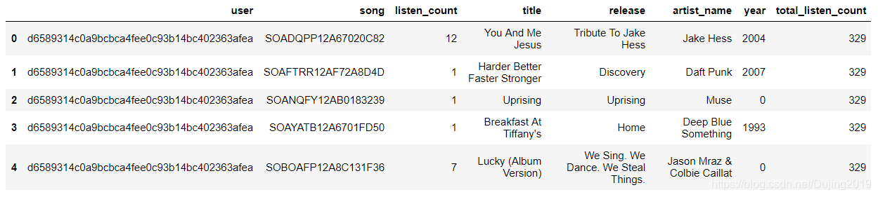
数据处理完毕，来看看它长什么样子吧

triplet_dataset_sub_song_merged.head(n=10)

现在的数据看起来工整多了，不光有用户对某个音乐作品的播放量，还有该音乐作品的名字和发布专辑，以及作者名字和发布时间。 现在我们只是大体了解了数据中各个指标的含义，对其具体内容还没有加以分析，一个新用户来了不知道给他推荐什么好，这时候就可以利用排行榜单了。可以统计最受欢迎的歌曲和歌手是哪些：

展示最流行的歌曲

import matplotlib.pyplot as plt; plt.rcdefaults()
import numpy as np
import matplotlib.pyplot as plt
#按歌曲名字来统计其播放量的总数
popular_songs = triplet_dataset_sub_song_merged[['title','listen_count']].groupby('title').sum().reset_index()
#对结果进行排序
popular_songs_top_20 = popular_songs.sort_values('listen_count', ascending=False).head(n=20)

#转换成list格式方便画图
objects = (list(popular_songs_top_20['title']))
#设置位置
y_pos = np.arange(len(objects))
#对应结果值
performance = list(popular_songs_top_20['listen_count'])
#绘图
plt.bar(y_pos, performance, align='center', alpha=0.5)
plt.xticks(y_pos, objects, rotation='vertical')
plt.ylabel('Item count')
plt.title('Most popular songs')
 
plt.show()

最受欢迎的releases

#按专辑名字来统计播放总量
popular_release = triplet_dataset_sub_song_merged[['release','listen_count']].groupby('release').sum().reset_index()
#排序
popular_release_top_20 = popular_release.sort_values('listen_count', ascending=False).head(n=20)

objects = (list(popular_release_top_20['release']))
y_pos = np.arange(len(objects))
performance = list(popular_release_top_20['listen_count'])
#绘图 
plt.bar(y_pos, performance, align='center', alpha=0.5)
plt.xticks(y_pos, objects, rotation='vertical')
plt.ylabel('Item count')
plt.title('Most popular Release')
 
plt.show()

最受欢迎的歌手

#按歌手来统计其播放总量
popular_artist = triplet_dataset_sub_song_merged[['artist_name','listen_count']].groupby('artist_name').sum().reset_index()
#排序
popular_artist_top_20 = popular_artist.sort_values('listen_count', ascending=False).head(n=20)

objects = (list(popular_artist_top_20['artist_name']))
y_pos = np.arange(len(objects))
performance = list(popular_artist_top_20['listen_count'])
#绘图 
plt.bar(y_pos, performance, align='center', alpha=0.5)
plt.xticks(y_pos, objects, rotation='vertical')
plt.ylabel('Item count')
plt.title('Most popular Artists')
 
plt.show()

用户播放过歌曲量的分布

user_song_count_distribution = triplet_dataset_sub_song_merged[['user','title']].groupby('user').count().reset_index().sort_values(
by='title',ascending = False)
user_song_count_distribution.title.describe()

count 99996.000000
mean 107.749890
std 79.742561
min 1.000000
25% 53.000000
50% 89.000000
75% 141.000000
max 1189.000000
Name: title, dtype: float64

x = user_song_count_distribution.title
n, bins, patches = plt.hist(x, 50, facecolor='green', alpha=0.75)
plt.xlabel('Play Counts')
plt.ylabel('Num of Users')
plt.title(r'$\mathrm{Histogram\ of\ User\ Play\ Count\ Distribution}\ $')
plt.grid(True)
plt.show()

绝大多数用户播放歌曲的数量在100左右，关于数据的处理和介绍已经给大家都分析过了，接下来我们要做的就是构建一个能实际进行推荐的程序了。

开始构建推荐系统

import Recommenders as Recommenders
from sklearn.model_selection import train_test_split

最简单的推荐方式就是排行榜单了，这里我们创建了一个函数，需要我们传入的是原始数据，用户列名，待统计的指标（例如按歌曲名字，歌手名字，专辑名字。选择统计哪项指标得到的排行榜单）：

triplet_dataset_sub_song_merged_set = triplet_dataset_sub_song_merged
train_data, test_data = train_test_split(triplet_dataset_sub_song_merged_set, test_size = 0.40, random_state=0)

train_data.head()

def create_popularity_recommendation(train_data, user_id, item_id):
    #根据指定的特征来统计其播放情况，可以选择歌曲名，专辑名，歌手名
    train_data_grouped = train_data.groupby([item_id]).agg({user_id: 'count'}).reset_index()
    #为了直观展示，我们用得分来表示其结果
    train_data_grouped.rename(columns = {user_id: 'score'},inplace=True)
    
    #排行榜单需要排序
    train_data_sort = train_data_grouped.sort_values(['score', item_id], ascending = [0,1])
    
    #加入一项排行等级，表示其推荐的优先级
    train_data_sort['Rank'] = train_data_sort['score'].rank(ascending=0, method='first')
        
    #返回指定个数的推荐结果
    popularity_recommendations = train_data_sort.head(20)
    return popularity_recommendations

recommendations = create_popularity_recommendation(triplet_dataset_sub_song_merged,'user','title')

得到推荐结果

recommendations

返回了一份前20的歌曲排行榜单，其中的得分这里只是进行了简单的播放计算，在设计的时候也可以综合考虑更多的指标，比如综合计算歌曲发布年份，歌手的流行程度等。

基于歌曲相似度的推荐

接下来就要进行相似度的计算来推荐歌曲了，为了加快代码的运行速度，选择了其中一部分数据来进行实验。

song_count_subset = song_count_df.head(n=5000)
user_subset = list(play_count_subset.user)
song_subset = list(song_count_subset.song)
triplet_dataset_sub_song_merged_sub = triplet_dataset_sub_song_merged[triplet_dataset_sub_song_merged.song.isin(song_subset)]

triplet_dataset_sub_song_merged_sub.head()

计算相似度得到推荐结果

import Recommenders as Recommenders
train_data, test_data = train_test_split(triplet_dataset_sub_song_merged_sub, test_size = 0.30, random_state=0)
is_model = Recommenders.item_similarity_recommender_py()
is_model.create(train_data, 'user', 'title')
user_id = list(train_data.user)[7]
user_items = is_model.get_user_items(user_id)

首先我们要针对某一个用户进行推荐，那必然得先得到他都听过哪些歌曲，通过这些已被听过的歌曲跟整个数据集中的歌曲进行对比，看哪些歌曲跟用户已听过的比较类似，推荐的就是这些类似的。如何计算呢？例如当前用户听过了66首歌曲，整个数据集中有4879个歌曲，我们要做的就是构建一个[66,4879]的矩阵，其中每一个值表示用户听过的每一个歌曲和数据集中每一个歌曲的相似度。这里使用Jaccard相似系数，矩阵中[i,j]的含义就是用户听过的第i首歌曲这些歌曲被哪些人听过，比如有3000人听过，数据集中的j歌曲被哪些人听过，比如有5000人听过。Jaccard相似系数就要求：
$Jaccard=\frac{交集(听过i歌曲的3000人和听过j歌曲的5000人)}{并集(听过i歌曲的3000人和听过j歌曲的5000人)}$
就是如果两个歌曲很相似，那其受众应当是一致的，交集/并集的比例应该比较大，如果两个歌曲没啥相关性，其值应当就比较小了。 上述代码中计算了矩阵[66,4879]中每一个位置的值应当是多少，在最后推荐的时候我们还应当注意一件事对于数据集中每一个待推荐的歌曲都需要跟该用户所有听过的歌曲计算其Jaccard值，例如歌曲j需要跟用户听过的66个歌曲计算其值，最终是否推荐的得分值还得进行处理，即把这66个值加在一起，最终求一个平均值，来代表该歌曲的推荐得分。

#执行推荐
is_model.recommend(user_id)

No. of unique songs for the user: 66
no. of unique songs in the training set: 4879
Non zero values in cooccurence_matrix :290327

基于矩阵分解（SVD）的推荐

triplet_dataset_sub_song_merged_sum_df = triplet_dataset_sub_song_merged[['user','listen_count']].groupby('user').sum().reset_index()
triplet_dataset_sub_song_merged_sum_df.rename(columns={'listen_count':'total_listen_count'},inplace=True)
triplet_dataset_sub_song_merged = pd.merge(triplet_dataset_sub_song_merged,triplet_dataset_sub_song_merged_sum_df)
triplet_dataset_sub_song_merged.head()

triplet_dataset_sub_song_merged['fractional_play_count'] = triplet_dataset_sub_song_merged['listen_count']/triplet_dataset_sub_song_merged['total_listen_count']

triplet_dataset_sub_song_merged[triplet_dataset_sub_song_merged.user =='d6589314c0a9bcbca4fee0c93b14bc402363afea'][['user','song','listen_count','fractional_play_count']].head()

from scipy.sparse import coo_matrix

small_set = triplet_dataset_sub_song_merged
user_codes = small_set.user.drop_duplicates().reset_index()
song_codes = small_set.song.drop_duplicates().reset_index()
user_codes.rename(columns={'index':'user_index'}, inplace=True)
song_codes.rename(columns={'index':'song_index'}, inplace=True)
song_codes['so_index_value'] = list(song_codes.index)
user_codes['us_index_value'] = list(user_codes.index)
small_set = pd.merge(small_set,song_codes,how='left')
small_set = pd.merge(small_set,user_codes,how='left')
mat_candidate = small_set[['us_index_value','so_index_value','fractional_play_count']]
data_array = mat_candidate.fractional_play_count.values
row_array = mat_candidate.us_index_value.values
col_array = mat_candidate.so_index_value.values

data_sparse = coo_matrix((data_array, (row_array, col_array)),dtype=float)

data_sparse

<99996x30000 sparse matrix of type ‘<class ‘numpy.float64’>’
with 10774558 stored elements in COOrdinate format>

上面代码先根据用户进行分组，计算每个用户的总的播放总量，然后用每首歌的播放总量相处，得到每首歌的分值，最后一列特征fractional_play_count就是用户对每首歌曲的评分值。 有了评分值之后就可以来构建矩阵了，这里有一些小问题需要处理一下，原始数据中无论是用户ID还是歌曲ID都是很长一串，这表达起来不太方便，需要重新对其制作索引。

user_codes[user_codes.user =='2a2f776cbac6df64d6cb505e7e834e01684673b6']

使用SVD方法来进行矩阵分解
矩阵构造好了之后我们就要执行SVD矩阵分解了，这里还需要一些额外的工具包来帮助我们完成计算，scipy就是其中一个好帮手了，里面已经封装好了SVD计算方法。

import math as mt
from scipy.sparse.linalg import * #used for matrix multiplication
from scipy.sparse.linalg import svds
from scipy.sparse import csc_matrix

def compute_svd(urm, K):
    U, s, Vt = svds(urm, K)

    dim = (len(s), len(s))
    S = np.zeros(dim, dtype=np.float32)
    for i in range(0, len(s)):
        S[i,i] = mt.sqrt(s[i])

    U = csc_matrix(U, dtype=np.float32)
    S = csc_matrix(S, dtype=np.float32)
    Vt = csc_matrix(Vt, dtype=np.float32)
    
    return U, S, Vt

def compute_estimated_matrix(urm, U, S, Vt, uTest, K, test):
    rightTerm = S*Vt 
    max_recommendation = 250
    estimatedRatings = np.zeros(shape=(MAX_UID, MAX_PID), dtype=np.float16)
    recomendRatings = np.zeros(shape=(MAX_UID,max_recommendation ), dtype=np.float16)
    for userTest in uTest:
        prod = U[userTest, :]*rightTerm
        estimatedRatings[userTest, :] = prod.todense()
        recomendRatings[userTest, :] = (-estimatedRatings[userTest, :]).argsort()[:max_recommendation]
    return recomendRatings

在执行SVD的时候需要我们额外指定一个指标K值，其含义就是我们选择前多少个特征值来做近似代表，也就是S矩阵中的数量。如果K值较大整体的计算效率会慢一些但是会更接近真实结果，这个值还需要我们自己来衡量一下。

K=50
urm = data_sparse
MAX_PID = urm.shape[1]
MAX_UID = urm.shape[0]

U, S, Vt = compute_svd(urm, K)

这里我们选择K值等于50，其中PID表示我们最开始选择的部分歌曲，UID表示我们选择的部分用户。

接下来我们需要选择待测试用户了：

uTest = [4,5,6,7,8,873,23]

随便选择一些用户就好，这里表示用户的索引编号，接下来需要对每一个用户计算其对我们候选集中3W首歌曲的喜好程度，就是估计他对这3W首歌的评分值应该等于多少，前面我们通过SVD矩阵分解已经计算所需各个小矩阵了，接下来把其还原回去就可以啦：

uTest = [4,5,6,7,8,873,23]

uTest_recommended_items = compute_estimated_matrix(urm, U, S, Vt, uTest, K, True)

for user in uTest:
    print("当前待推荐用户编号 {}". format(user))
    rank_value = 1
    for i in uTest_recommended_items[user,0:10]:
        song_details = small_set[small_set.so_index_value == i].drop_duplicates('so_index_value')[['title','artist_name']]
        print("推荐编号： {} 推荐歌曲： {} 作者： {}".format(rank_value, list(song_details['title'])[0],list(song_details['artist_name'])[0]))
        rank_value+=1

当前待推荐用户编号 4
推荐编号： 1 推荐歌曲： Fireflies 作者： Charttraxx Karaoke
推荐编号： 2 推荐歌曲： Hey_ Soul Sister 作者： Train
推荐编号： 3 推荐歌曲： OMG 作者： Usher featuring will.i.am
推荐编号： 4 推荐歌曲： Lucky (Album Version) 作者： Jason Mraz & Colbie Caillat
推荐编号： 5 推荐歌曲： Vanilla Twilight 作者： Owl City
推荐编号： 6 推荐歌曲： Crumpshit 作者： Philippe Rochard
推荐编号： 7 推荐歌曲： Billionaire [feat. Bruno Mars] (Explicit Album Version) 作者： Travie McCoy
推荐编号： 8 推荐歌曲： Love Story 作者： Taylor Swift
推荐编号： 9 推荐歌曲： TULENLIEKKI 作者： M.A. Numminen
推荐编号： 10 推荐歌曲： Use Somebody 作者： Kings Of Leon
当前待推荐用户编号 5
推荐编号： 1 推荐歌曲： Sehr kosmisch 作者： Harmonia
推荐编号： 2 推荐歌曲： Ain’t Misbehavin 作者： Sam Cooke
推荐编号： 3 推荐歌曲： Dog Days Are Over (Radio Edit) 作者： Florence + The Machine
推荐编号： 4 推荐歌曲： Revelry 作者： Kings Of Leon
推荐编号： 5 推荐歌曲： Undo 作者： Björk
推荐编号： 6 推荐歌曲： Cosmic Love 作者： Florence + The Machine
推荐编号： 7 推荐歌曲： Home 作者： Edward Sharpe & The Magnetic Zeros
推荐编号： 8 推荐歌曲： You’ve Got The Love 作者： Florence + The Machine
推荐编号： 9 推荐歌曲： Bring Me To Life 作者： Evanescence
推荐编号： 10 推荐歌曲： Tighten Up 作者： The Black Keys
当前待推荐用户编号 6
推荐编号： 1 推荐歌曲： Crumpshit 作者： Philippe Rochard
推荐编号： 2 推荐歌曲： Marry Me 作者： Train
推荐编号： 3 推荐歌曲： Hey_ Soul Sister 作者： Train
推荐编号： 4 推荐歌曲： Lucky (Album Version) 作者： Jason Mraz & Colbie Caillat
推荐编号： 5 推荐歌曲： One On One 作者： the bird and the bee
推荐编号： 6 推荐歌曲： I Never Told You 作者： Colbie Caillat
推荐编号： 7 推荐歌曲： Canada 作者： Five Iron Frenzy
推荐编号： 8 推荐歌曲： Fireflies 作者： Charttraxx Karaoke
推荐编号： 9 推荐歌曲： TULENLIEKKI 作者： M.A. Numminen
推荐编号： 10 推荐歌曲： Bring Me To Life 作者： Evanescence
当前待推荐用户编号 7
推荐编号： 1 推荐歌曲： Behind The Sea [Live In Chicago] 作者： Panic At The Disco
推荐编号： 2 推荐歌曲： The City Is At War (Album Version) 作者： Cobra Starship
推荐编号： 3 推荐歌曲： Dead Souls 作者： Nine Inch Nails
推荐编号： 4 推荐歌曲： Una Confusion 作者： LU
推荐编号： 5 推荐歌曲： Home 作者： Edward Sharpe & The Magnetic Zeros
推荐编号： 6 推荐歌曲： Climbing Up The Walls 作者： Radiohead
推荐编号： 7 推荐歌曲： Tighten Up 作者： The Black Keys
推荐编号： 8 推荐歌曲： Tive Sim 作者： Cartola
推荐编号： 9 推荐歌曲： West One (Shine On Me) 作者： The Ruts
推荐编号： 10 推荐歌曲： Cosmic Love 作者： Florence + The Machine
当前待推荐用户编号 8
推荐编号： 1 推荐歌曲： Undo 作者： Björk
推荐编号： 2 推荐歌曲： Canada 作者： Five Iron Frenzy
推荐编号： 3 推荐歌曲： Better To Reign In Hell 作者： Cradle Of Filth
推荐编号： 4 推荐歌曲： Unite (2009 Digital Remaster) 作者： Beastie Boys
推荐编号： 5 推荐歌曲： Behind The Sea [Live In Chicago] 作者： Panic At The Disco
推荐编号： 6 推荐歌曲： Rockin’ Around The Christmas Tree 作者： Brenda Lee
推荐编号： 7 推荐歌曲： Devil’s Slide 作者： Joe Satriani
推荐编号： 8 推荐歌曲： Revelry 作者： Kings Of Leon
推荐编号： 9 推荐歌曲： 16 Candles 作者： The Crests
推荐编号： 10 推荐歌曲： Catch You Baby (Steve Pitron & Max Sanna Radio Edit) 作者： Lonnie Gordon
当前待推荐用户编号 873
推荐编号： 1 推荐歌曲： The Scientist 作者： Coldplay
推荐编号： 2 推荐歌曲： Yellow 作者： Coldplay
推荐编号： 3 推荐歌曲： Clocks 作者： Coldplay
推荐编号： 4 推荐歌曲： Fix You 作者： Coldplay
推荐编号： 5 推荐歌曲： In My Place 作者： Coldplay
推荐编号： 6 推荐歌曲： Shiver 作者： Coldplay
推荐编号： 7 推荐歌曲： Speed Of Sound 作者： Coldplay
推荐编号： 8 推荐歌曲： Creep (Explicit) 作者： Radiohead
推荐编号： 9 推荐歌曲： Sparks 作者： Coldplay
推荐编号： 10 推荐歌曲： Use Somebody 作者： Kings Of Leon
当前待推荐用户编号 23
推荐编号： 1 推荐歌曲： Garden Of Eden 作者： Guns N’ Roses
推荐编号： 2 推荐歌曲： Don’t Speak 作者： John Dahlbäck
推荐编号： 3 推荐歌曲： Master Of Puppets 作者： Metallica
推荐编号： 4 推荐歌曲： TULENLIEKKI 作者： M.A. Numminen
推荐编号： 5 推荐歌曲： Bring Me To Life 作者： Evanescence
推荐编号： 6 推荐歌曲： Kryptonite 作者： 3 Doors Down
推荐编号： 7 推荐歌曲： Make Her Say 作者： Kid Cudi / Kanye West / Common
推荐编号： 8 推荐歌曲： Night Village 作者： Deep Forest
推荐编号： 9 推荐歌曲： Better To Reign In Hell 作者： Cradle Of Filth
推荐编号： 10 推荐歌曲： Xanadu 作者： Olivia Newton-John;Electric Light Orchestra

这里对每一个用户都得到了其对应的推荐结果，并且将结果按照得分值进行排序。

我们选择了音乐数据集来进行个性化推荐任务，首先对数据进行预处理和整合，选择两种方法分别完成推荐任务。在相似度计算中根据用户所听过的歌曲在候选集中选择与其最相似的歌曲，存在的问题就是计算时间消耗太多，每一个用户都需要重新计算一遍才能得出推荐结果。在SVD矩阵分解的方法中，我们首先构建评分矩阵，对其进行SVD分解，然后选择待推荐用户，还原得到其对所有歌曲的估测评分值，最后排序返回结果即可。

uTest = [27513]
uTest_recommended_items = compute_estimated_matrix(urm, U, S, Vt, uTest, K, True)

for user in uTest:
    print("当前待推荐用户编号 {}". format(user))
    rank_value = 1
    for i in uTest_recommended_items[user,0:10]:
        song_details = small_set[small_set.so_index_value == i].drop_duplicates('so_index_value')[['title','artist_name']]
        print("推荐编号： {} 推荐歌曲： {} 作者： {}".format(rank_value, list(song_details['title'])[0],list(song_details['artist_name'])[0]))
        rank_value+=1

Recommendation for user with user id 27513
The number 1 recommended song is Master Of Puppets BY Metallica
The number 2 recommended song is Garden Of Eden BY Guns N’ Roses
The number 3 recommended song is Bring Me To Life BY Evanescence
The number 4 recommended song is Kryptonite BY 3 Doors Down
The number 5 recommended song is Make Her Say BY Kid Cudi / Kanye West / Common
The number 6 recommended song is Night Village BY Deep Forest
The number 7 recommended song is Savior BY Rise Against
The number 8 recommended song is Good Things BY Rich Boy / Polow Da Don / Keri Hilson
The number 9 recommended song is Bleed It Out [Live At Milton Keynes] BY Linkin Park
The number 10 recommended song is Uprising BY Muse