参考tensorflow2.0官网图像分类教程：https://tensorflow.google.cn/tutorials/keras/classification

一、数据集

1.1、Fashion MNIST介绍

该数据集包含10个类别中的70,000个灰度图像。图像显示了低分辨率（28 x 28像素）的单件服装

1.2、导入数据集

import tensorflow as tf
from tensorflow import keras

import numpy as np
import matplotlib.pyplot as plt

print(tf.__version__)
print(keras.__version__)

# 导入fashion MNIST 数据集
fashion_mnist = keras.datasets.fashion_mnist
# 训练集、训练标签；测试集、测试标签
(train_images, train_labels), (test_images, test_lables) = fashion_mnist.load_data()


print(train_images.shape)   # (60000, 28, 28)
print(train_labels.shape)   # (60000,)
print(test_images.shape)    # (10000, 28, 28)
print(test_lables.shape)    # (10000,)

图像是28x28 NumPy数组，像素值介于0到255之间。标签是一个整数数组，范围从0到9.这些对应于图像所代表的服装类别：
在这里插入图片描述
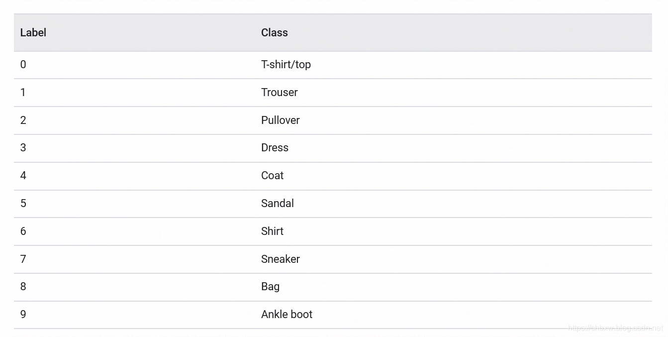
标签类名：

class_names = ['T-shirt/top', 'Trouser', 'Pullover', 'Dress', 'Coat',
               'Sandal', 'Shirt', 'Sneaker', 'Bag', 'Ankle boot']

查看图像

plt.figure()
plt.subplot(1, 2, 1)
plt.imshow(train_images[0])
plt.colorbar()
plt.grid(False)

# 归一化， 像素值都在0~255
train_images = train_images / 255.0
test_images = test_images / 255.0

plt.subplot(1, 2, 2)
plt.imshow(train_images[0], cmap=plt.cm.binary)
plt.colorbar()
plt.grid(False)
plt.show()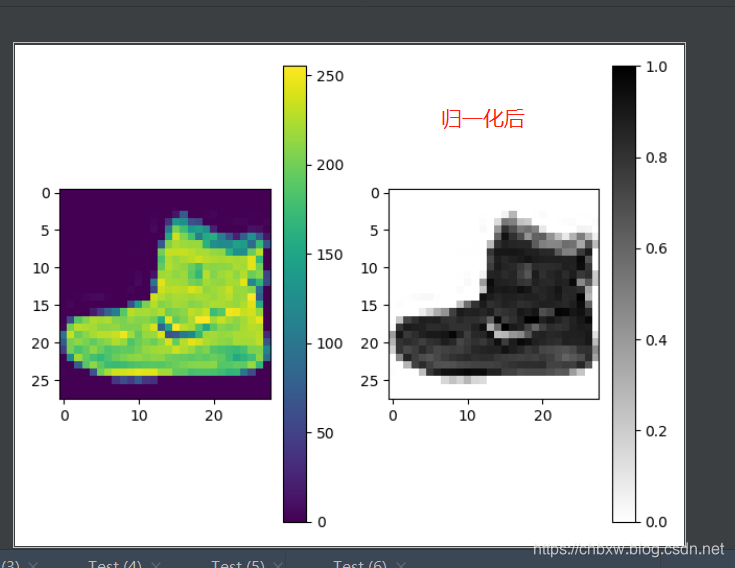

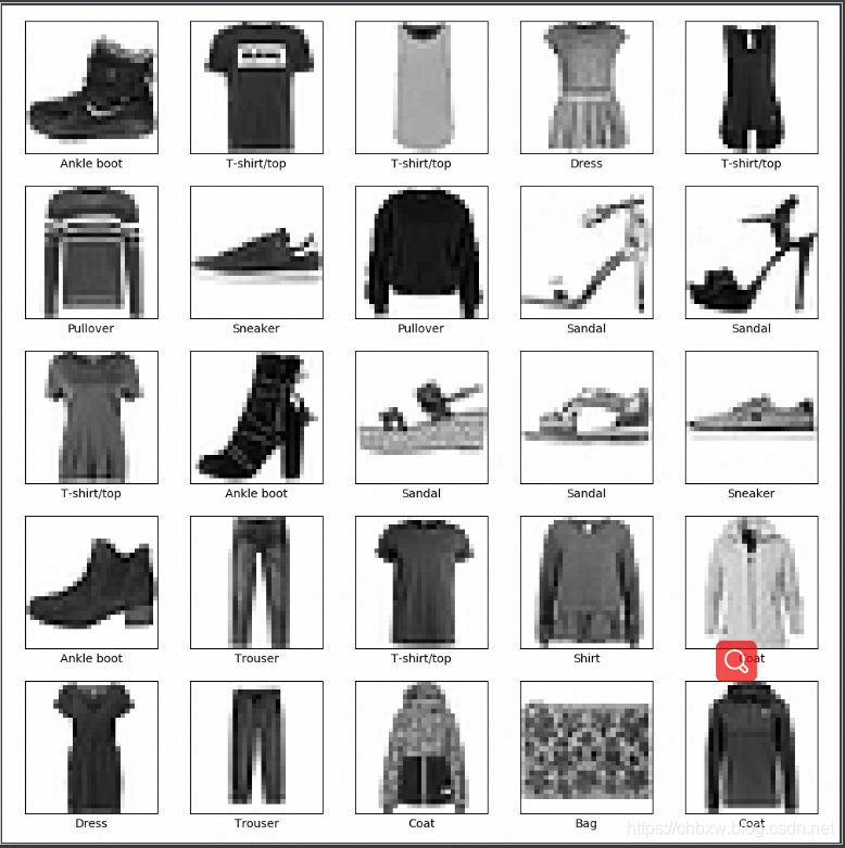
在这里插入图片描述

验证数据集标签的正确性，查看一下前25张图片，将标签显示在图片的下方

在这里插入图片描述

二、建模

2.1、构造层(set up layers)

神经网络的基本构件是层(layer)，层从输入数据提取表现(representations), 希望这些表现能够对现有问题有所帮助。
很多深度学习有许多简单的层链接在一起的，许多层拥有在训练中学习的参数，例如tf.keras.layers.Dense。

model = keras.Sequential([
    keras.layers.Flatten(input_shape=(28, 28)),
    keras.layers.Dense(128, activation='relu'),
    keras.layers.Dense(10, activation='softmax')
])

第一层，转换图像格式：将二维(28*28)的图像数组转为一维(28*28=784)，这层没有学习参数，只是格式数据。
在像素被压平(flatten)之后,接下来是两个keras.layers.Dense层，它们是紧密连接、或完全连接的神经层。
第二层，128个节点(nodes or neurons) 。
第三层，10个节点的softmax层，输出10个可能的分数，加在一起和为1，表示10个分类的可能性分数
激活函数：relu，softmax

2.2、编译模型(Compile the model)

在训练模型前，有一些设置需要在编译模型：

Loss function —This measures how accurate the model is during training. You want to minimize this function to “steer” the model in the right direction.
Optimizer —This is how the model is updated based on the data it sees and its loss function.
Metrics —Used to monitor the training and testing steps. The following example uses accuracy, the fraction of the images that are correctly classified.

# 编译模型
model.compile(optimizer='adam',
              loss='sparse_categorical_crossentropy',
              metrics=['accuracy'])

三、训练模型

训练神经网络模型需要以下步骤:

扫描二维码关注公众号，回复： 8539208 查看本文章

1、将训练数据输入模型，本例中的图像和标签
2、模型学习将图像和标签联系起来
3、通过测试集验证模型的准确性

3.1、训练

# 训练模型
model.fit(train_images, train_labels, epochs=10)

模型训练中，显示loss,accuracy
56352/60000 [===========================>..] - ETA: 0s - loss: 0.2497 - accuracy: 0.9059
57024/60000 [===========================>..] - ETA: 0s - loss: 0.2501 - accuracy: 0.9057
57760/60000 [===========================>..] - ETA: 0s - loss: 0.2500 - accuracy: 0.9059
58528/60000 [============================>.] - ETA: 0s - loss: 0.2496 - accuracy: 0.9059
59264/60000 [============================>.] - ETA: 0s - loss: 0.2501 - accuracy: 0.9057

3.2、评估准确性

# 评估模型， 使用测试集评估
test_loss, test_acc = model.evaluate(test_images,  test_labels, verbose=2)
print('\nTest accuracy:', test_acc)

# 10000/1 - 1s - loss: 0.2630 - accuracy: 0.8757
# Test accuracy: 0.8757

四、预测

# 预测
predictions = model.predict(test_images)

print(predictions[0]) # 10个评分，表示10个分类的可能性
# [3.1136313e-08 3.8150518e-09 1.1725315e-10 9.5243632e-11 1.9169266e-10
#  6.1769143e-04 2.1648395e-08 3.2574847e-02 2.0015452e-07 9.6680719e-01]

# 预测值与标签值
print(np.argmax(predictions[0]), test_labels[0])    # 9, 9

4.2、通过绘制图像显示10个分类

def plot_image(i, predictions_array, true_label, img):
    predictions_array, true_label, img = predictions_array, true_label[i], img[i]
    plt.grid(False)
    plt.xticks([])
    plt.yticks([])

    plt.imshow(img, cmap=plt.cm.binary)

    predicted_label = np.argmax(predictions_array)
    if predicted_label == true_label:
        color = 'blue'
    else:
        color = 'red'

    plt.xlabel("{} {:2.0f}% ({})".format(class_names[predicted_label],
                                         100*np.max(predictions_array),
                                         class_names[true_label]),
               color=color)

def plot_value_array(i, predictions_array, true_label):
    predictions_array, true_label = predictions_array, true_label[i]
    plt.grid(False)
    plt.xticks(range(10))
    plt.yticks([])
    thisplot = plt.bar(range(10), predictions_array, color="#777777")
    plt.ylim([0, 1])
    predicted_label = np.argmax(predictions_array)

    thisplot[predicted_label].set_color('red')
    thisplot[true_label].set_color('blue')

4.2.1、显示第一个图像

正确预测标签显示蓝色，错误预测标签显示红色

i = 0
plt.figure(figsize=(6,3))
plt.subplot(1,2,1)
plot_image(i, predictions[i], test_labels, test_images)
plt.subplot(1,2,2)
plot_value_array(i, predictions[i],  test_labels)
plt.show()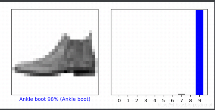

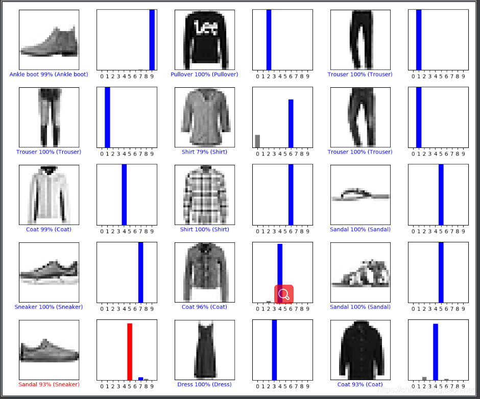
在这里插入图片描述

4.2.2、显示更多图片的预测

num_rows = 5
num_cols = 3
num_images = num_rows*num_cols
plt.figure(figsize=(2*2*num_cols, 2*num_rows))
for i in range(num_images):
    plt.subplot(num_rows, 2*num_cols, 2*i+1)
    plot_image(i, predictions[i], test_labels, test_images)
    plt.subplot(num_rows, 2*num_cols, 2*i+2)
    plot_value_array(i, predictions[i], test_labels)
plt.tight_layout()
plt.show()