玩了那么多天,终于有时间来写博客了.之前看过很多TensorFlow官网地址的教程,全忘了.现在复习,就从头开始吧,加油!
一.载入Fashion MNIST数据集
首先介绍一下Fashion MNIST数据集,它是7万张灰度图像组成,可以分成10个类别.每个灰度图像都是28*28像素的图像.我们将使用其中的6万张进行训练网络,另外的1万张来评估准确率.你可以直接使用TensorFlow来引入载入数据,代码如下:(注意这里要求的TensorFlow的版本在1.8.0之上,因为我之前的版本是1.7.0,就无法运行这个代码,打开终端,使用source activate tensorflow来激活TensorFlow,,再运行命令 pip install --upgrade tensorflow来更新TensorFlow.)
上面代码的运行结果是:Fashion MNIST数据集被下载在地址:/root/.keras/datasets/fashion-mnist,其下存在四个gz文件,分别代表的训练集特征和标签,测试集特征和标签.每个图像是一个28×28的numpy数组,每个像素值在0到255之间.标签在0-9之间,代表着衣服的类型.
| label | class |
| 0 | T-shirt/top |
| 1 | Trouser |
| 2 | Pullover |
| 3 | Dress |
| 4 | Coat |
| 5 | Sandal |
| 6 | Skirt |
| 7 | Sneaker |
| 8 | Bag |
| 9 | ankle boot |
下载数据的代码:(TensorFlow版本至少要求1.8.0,否则提示keras.datasets.fashion_mnist没有模块load_data())
import tensorflow as tf
from tensorflow import keras

import numpy as np
import matplotlib.pyplot as plt

fashion_mnist = keras.datasets.fashion_mnist

(train_images, train_labels), (test_images, test_labels) = fashion_mnist.load_data()
实验的结果:下载了四个gz文档在/root/.keras/datasets下.
除此之外,我们还需要在代码上补充一下每个类别的名称,组成一个list,代码如下:
class_names=['T-shirt/top','Trouser','Pullover','Dress','Coat',
             'Sandal','Shirt','Sneaker','Bag','Ankle boot']
二.探索数据,比如说shape等等
之前说过,我们的训练集由6万张28*28像素的图像组成,所以可以得到训练集的特征的大小是(60000,28,28),同样的训练集的标签的大小是(60000,),每一个标签是0-9之间的一个整数.测试集是由1万张28*28像素的图像组成的,所以它的大小是(10000,28,28),测试集的标签的大小是10000.
详见代码如下:
print("The shape of train_images is ",train_images.shape)
print("The shape of train_labels is ",train_labels.shape)
print("The shape of test_images is ",test_images.shape)
print("The length of test_labels is ",len(test_labels))
答案如下:
The shape of train_images is  (60000, 28, 28)
The shape of train_labels is  (60000,)
The shape of test_images is  (10000, 28, 28)
The length of test_labels is  10000
三.预处理数据
首先我们可视化第一个训练集的样本,使用的是matplotlib进行绘图,很显然,你可以看到它的每一个像素值都在0-255之间,不知道你有没有有学习过吴恩达机器学习的课程,他有讲过关于数据归一化的操作(将每一个值规模改成0-1之间,或者-1到1之间,这里我们改成0-1之间.).这里我简单的介绍一下归一化的原因:简化问题,比如说对于二维的分类问题,只受两个特征影响的分类,一个特征的范围在0-2之间,但是另一个特征的范围在2000-4000之间,这个分类问题可以简单的使用一条直线进行分类,很显然对于线性来说,我的第二个特征的影响更大,更何况二次方三次方之后等等,所以进行归一化.
可视化原始数据的代码:(仅仅展示第一个样本的数据)
plt.figure()
plt.imshow(train_images[0])
plt.colorbar()
plt.gca().grid(False)
plt.show()
首先将我们的特征的值从整数变成浮点数,其次我们在除以255.
代码如下:
train_images=train_images/255.0
test_images=test_images/255.0
可视化归一化之后的数据的代码:
plt.figure(figsize=(10,10))
for i in range(25):
    plt.subplot(5,5,i+1)
    plt.xticks([])
    plt.yticks([])
    plt.grid('off')
    plt.imshow(train_images[i],cmap=plt.cm.binary)
    plt.xlabel(class_names[train_labels[i]])
plt.show()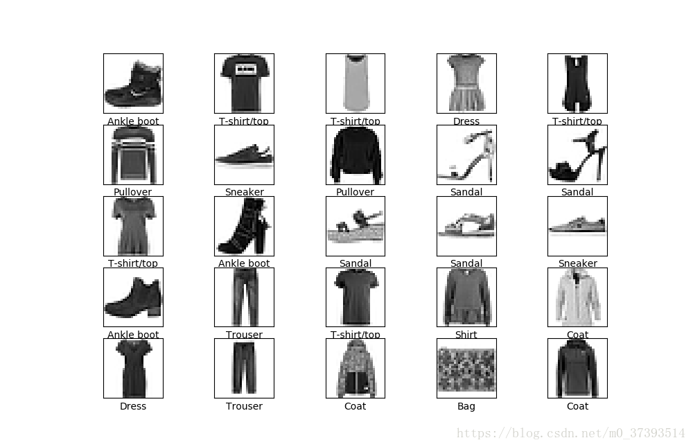
四.构建模型
4.1 配置层
代码:
model=keras.Sequential([
    keras.layers.Flatten(input_shape=(28,28)),
    keras.layers.Dense(128,activation=tf.nn.relu),
    keras.layers.Dense(10,activation=tf.nn.softmax)
])
代码解析:
上面的代码很显然存在三层,其中第一层是tf.keras.layers.Flatten(),主要的功能就是将(28,28)像素的图像即对应的2维的数组转成28*28=784的一维的数组.第二层是Dense,如果你上过吴恩达的课程,或者有一点机器学习的基础的话,这个可以理解成全连接层,这个层存在128的神经元.最后一层是softmax层,它返回的是由10个概率值(加起来等于1)组成的1维数组,每一个代表了这个图像属于某个类别的概率.
4.2 编译模型
代码:
model.compile(optimizer=tf.train.AdamOptimizer(),
              loss='sparse_categorical_crossentropy',
              metrics=['accuracy'])
代码解析:
优化器是AdamOptimizer(表示采用何种方式寻找最佳答案,有什么梯度下降啊等等),损失函数是sparse_categorical_crossentropy(就是损失函数怎么定义的,最佳值就是使得损失函数最小).计量标准是准确率,也就是正确归类的图像的概率.
五.训练模型
为了开始训练,我们调用函数model.fit,训练为5次.当模型训练的时候,损失和准确率展示如下,在训练集上达到88%的准确率.
代码:
model.fit(train_images,train_labels,epochs=5)结果:(仅仅截取了最后的那一个)
Epoch 1/5
60000/60000 [==============================] - 8s 132us/step - loss: 0.4957 - acc: 0.8247
Epoch 2/5
60000/60000 [==============================] - 7s 114us/step - loss: 0.3723 - acc: 0.8657
Epoch 3/5
60000/60000 [==============================] - 7s 118us/step - loss: 0.3365 - acc: 0.8779
Epoch 4/5
60000/60000 [==============================] - 7s 115us/step - loss: 0.3117 - acc: 0.8854
Epoch 5/5
60000/60000 [==============================] - 7s 116us/step - loss: 0.2958 - acc: 0.8908
六.评估准确率
在测试集上完成准确率的评估,调用的是model.evaluate()
代码:
test_loss,test_acc=model.evaluate(test_images,test_labels)
print('Test Acc:',test_acc)
结果:
 32/10000 [..............................] - ETA: 10s
 1056/10000 [==>...........................] - ETA: 0s
 1760/10000 [====>.........................] - ETA: 0s
 2432/10000 [======>.......................] - ETA: 0s
 3200/10000 [========>.....................] - ETA: 0s
 4192/10000 [===========>..................] - ETA: 0s
 4928/10000 [=============>................] - ETA: 0s
 5888/10000 [================>.............] - ETA: 0s
 6624/10000 [==================>...........] - ETA: 0s
 7360/10000 [=====================>........] - ETA: 0s
 8256/10000 [=======================>......] - ETA: 0s
 9056/10000 [==========================>...] - ETA: 0s
 9856/10000 [============================>.] - ETA: 0s
10000/10000 [==============================] - 1s 65us/step
Test Acc: 0.8692
这儿的准确率是86.9%,比之前的训练集的准确率低,之间的差距可以理解成是一种过拟合的现象,它是机器学习的常遇到的问题,指的是对训练的模型对训练数据准确率很高,但是应用到新的数据的时候,出现了不好的结果.
七.进行预测
对所有的测试集的数据进行预测,model.predict()返回的是一个list,我们每一个元素是对一个图像的预测结果,这个预测结果是一个一维的包含10个概率的数组,概率最大的元素的下标就是结果.
我们这里取的是第一个测试集样本进行结果展示:你会发现最大的概率下标是9,正确的所属类别下标也是9.
代码:
predictions=model.predict(test_images)
print("The first picture's prediction is:{},so the result is:{}".format(predictions[0],np.argmax(predictions[0])))
print("The first picture is ",test_labels[0])
结果:
The first picture's prediction is:[8.8176442e-08 1.0522982e-08 9.9359028e-08 4.4886299e-08 3.6108457e-08
 9.8875919e-03 3.0011483e-06 8.3239987e-02 6.6848101e-05 9.0680236e-01],so the result is:9
The first picture is  9
这里还绘制了前25个样本的预测结果和真是结果展示图,正确为绿色,不正确为红色.
代码:
plt.figure(figsize=(10, 10))
for i in range(25):
    plt.subplot(5, 5, i + 1)
    plt.xticks([])
    plt.yticks([])
    plt.grid('off')
    plt.imshow(test_images[i], cmap=plt.cm.binary)
    predicted_label = np.argmax(predictions[i])
    true_label = test_labels[i]
    if predicted_label == true_label:
        color = 'green'
    else:
        color = 'red'
    plt.xlabel("{} ({})".format(class_names[predicted_label],
                                class_names[true_label]),
               color=color)
plt.show()
结果:
/home/syq/anaconda3/envs/tensorflow/lib/python3.6/site-packages/matplotlib/cbook/deprecation.py:107: MatplotlibDeprecationWarning: Passing one of 'on', 'true', 'off', 'false' as a boolean is deprecated; use an actual boolean (True/False) instead.
  warnings.warn(message, mplDeprecation, stacklevel=1)
我们还可以只预测其中一个样本,拿第一个测试集样本举例,你会发现与之前的答案一致,都是9.
第一个空行前面的代码,是在数据集上取得一个样本,根据结果可以得到我们的图像是28*28像素的.---(28.28)
第二个空行前面的代码是为了什么呢?看第二部分我们知道,我们的数据集的大小,因为tf.keras模型对一批数据进行预测结果的优化,所以,我们对于单独的一张图片,我们需要将其加入list中,其实就是增加一个维度.---(1,28,28)
代码:
img=test_images[0]
print(img.shape)

img=(np.expand_dims(img,0))
print(img.shape)

predictions=model.predict(img)
print(predictions)

prediction=predictions[0]
print("You will find that the ans is same to the former res",np.argmax(prediction))
结果:
(28, 28)
(1, 28, 28)
[[8.8176598e-08 1.0522981e-08 9.9359013e-08 4.4886296e-08 3.6108588e-08
  9.8876050e-03 3.0011479e-06 8.3240032e-02 6.6848348e-05 9.0680224e-01]]
You will find that the ans is same to the former res 9