python图像处理二值化方法
1. opencv 简单阈值 cv2.threshold
2. opencv 自适应阈值 cv2.adaptiveThreshold
3. Otsu's 二值化
例子:
来自 : OpenCV-Python 中文教程
1 import cv2
2 import numpy as np
3 from matplotlib import pyplot as plt
4
5 img = cv2.imread('scratch.png', 0)
6 # global thresholding
7 ret1, th1 = cv2.threshold(img, 127, 255, cv2.THRESH_BINARY)
8 # Otsu's thresholding
9 th2 = cv2.adaptiveThreshold(img, 255, cv2.ADAPTIVE_THRESH_MEAN_C, cv2.THRESH_BINARY, 11, 2)
10 # Otsu's thresholding
11 # 阈值一定要设为 0 !
12 ret3, th3 = cv2.threshold(img, 0, 255, cv2.THRESH_BINARY + cv2.THRESH_OTSU)
13 # plot all the images and their histograms
14 images = [img, 0, th1, img, 0, th2, img, 0, th3]
15 titles = [
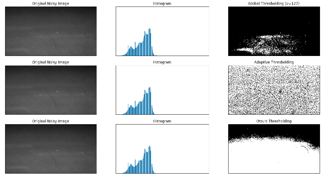
16 'Original Noisy Image', 'Histogram', 'Global Thresholding (v=127)',
17 'Original Noisy Image', 'Histogram', "Adaptive Thresholding",
18 'Original Noisy Image', 'Histogram', "Otsu's Thresholding"
19 ]
20 # 这里使用了 pyplot 中画直方图的方法, plt.hist, 要注意的是它的参数是一维数组
21 # 所以这里使用了( numpy ) ravel 方法,将多维数组转换成一维,也可以使用 flatten 方法
22 # ndarray.flat 1-D iterator over an array.
23 # ndarray.flatten 1-D array copy of the elements of an array in row-major order.
24 for i in range(3):
25 plt.subplot(3, 3, i * 3 + 1), plt.imshow(images[i * 3], 'gray')
26 plt.title(titles[i * 3]), plt.xticks([]), plt.yticks([])
27 plt.subplot(3, 3, i * 3 + 2), plt.hist(images[i * 3].ravel(), 256)
28 plt.title(titles[i * 3 + 1]), plt.xticks([]), plt.yticks([])
29 plt.subplot(3, 3, i * 3 + 3), plt.imshow(images[i * 3 + 2], 'gray')
30 plt.title(titles[i * 3 + 2]), plt.xticks([]), plt.yticks([])
31 plt.show()
结果图:
4. skimage niblack阈值
5. skimage sauvola阈值
例子:
https://scikit-image.org/docs/dev/auto_examples/segmentation/plot_niblack_sauvola.html
 1 import matplotlib
 2 import matplotlib.pyplot as plt
 3
 4 from skimage.data import page
 5 from skimage.filters import (threshold_otsu, threshold_niblack,
 6                              threshold_sauvola)
 7
 8
 9 matplotlib.rcParams['font.size'] = 9
10
11
12 image = page()
13 binary_global = image > threshold_otsu(image)
14
15 window_size = 25
16 thresh_niblack = threshold_niblack(image, window_size=window_size, k=0.8)
17 thresh_sauvola = threshold_sauvola(image, window_size=window_size)
18
19 binary_niblack = image > thresh_niblack
20 binary_sauvola = image > thresh_sauvola
21
22 plt.figure(figsize=(8, 7))
23 plt.subplot(2, 2, 1)
24 plt.imshow(image, cmap=plt.cm.gray)
25 plt.title('Original')
26 plt.axis('off')
27
28 plt.subplot(2, 2, 2)
29 plt.title('Global Threshold')
30 plt.imshow(binary_global, cmap=plt.cm.gray)
31 plt.axis('off')
32
33 plt.subplot(2, 2, 3)
34 plt.imshow(binary_niblack, cmap=plt.cm.gray)
35 plt.title('Niblack Threshold')
36 plt.axis('off')
37
38 plt.subplot(2, 2, 4)
39 plt.imshow(binary_sauvola, cmap=plt.cm.gray)
40 plt.title('Sauvola Threshold')
41 plt.axis('off')
42
43 plt.show()
结果图:

6.