本教程为脑机学习者Rose发表于公众号:脑机接口社区(微信号:Brain_Computer).QQ交流群:903290195

Raw数据结构
Raw对象主要用来存储连续型数据,核心数据为n_channels和times,也包含Info对象。
下面可以通过几个案例来说明Raw对象和相关用法。
Raw结构查看:
# 引入python库
import mne
from mne.datasets import sample
import matplotlib.pyplot as plt

# sample的存放地址
data_path = sample.data_path()
# 该fif文件存放地址
fname = data_path + '/MEG/sample/sample_audvis_raw.fif'

"""
如果上述给定的地址中存在该文件,则直接加载本地文件,
如果不存在则在网上下载改数据
"""
raw = mne.io.read_raw_fif(fname)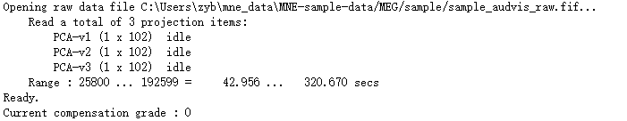
通过打印raw:
print(raw)
<Raw | sample_audvis_raw.fif, n_channels x n_times : 376 x 166800 (277.7 sec), ~3.6 MB, data not loaded>
可以看出核心数据为n_channels和n_times
raw.info<Info | 24 non-empty fields
acq_pars : str | 13886 items
bads : list | MEG 2443, EEG 053
ch_names : list | MEG 0113, MEG 0112, MEG 0111, MEG 0122, MEG 0123, ...
chs : list | 376 items (GRAD: 204, MAG: 102, STIM: 9, EEG: 60, EOG: 1)
comps : list | 0 items
custom_ref_applied : bool | False
description : str | 49 items
dev_head_t : Transform | 3 items
dig : Digitization | 146 items (3 Cardinal, 4 HPI, 61 EEG, 78 Extra)
events : list | 1 items
experimenter : str | 3 items
file_id : dict | 4 items
highpass : float | 0.10000000149011612 Hz
hpi_meas : list | 1 items
hpi_results : list | 1 items
lowpass : float | 172.17630004882812 Hz
meas_date : tuple | 2002-12-03 19:01:10 GMT
meas_id : dict | 4 items
nchan : int | 376
proc_history : list | 0 items
proj_id : ndarray | 1 items
proj_name : str | 4 items
projs : list | PCA-v1: off, PCA-v2: off, PCA-v3: off
sfreq : float | 600.614990234375 Hz
acq_stim : NoneType
ctf_head_t : NoneType
dev_ctf_t : NoneType
device_info : NoneType
gantry_angle : NoneType
helium_info : NoneType
hpi_subsystem : NoneType
kit_system_id : NoneType
line_freq : NoneType
subject_info : NoneType
utc_offset : NoneType
xplotter_layout : NoneType
上面为row中info的信息,从中可以看出info记录了raw中有哪些是不良通道(bads),通道名称:ch_names,sfreq:采样频率等。
通常raw的数据访问方式如下:
data, times = raw[picks, time_slice]
picks:是根据条件挑选出来的索引;
time_slice:时间切片
想要获取raw中所有数据,以下两种方式均可:
data,times=raw[:]
data,times=raw[:,:]
"""
案例:
获取10-20秒内的良好的MEG数据

# 根据type来选择 那些良好的MEG信号(良好的MEG信号,通过设置exclude="bads") channel,
结果为 channels所对应的的索引
"""

picks = mne.pick_types(raw.info, meg=True, exclude='bads')
t_idx = raw.time_as_index([10., 20.])
data, times = raw[picks, t_idx[0]:t_idx[1]]
plt.plot(times,data.T)
plt.title("Sample channels")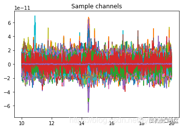
"""
sfreq:采样频率

raw返回所选信道以及时间段内的数据和时间点,
分别赋值给data以及times(即raw对象返回的是两个array)
"""
sfreq=raw.info['sfreq']
data,times=raw[:5,int(sfreq*1):int(sfreq*3)]
plt.plot(times,data.T)
plt.title("Sample channels")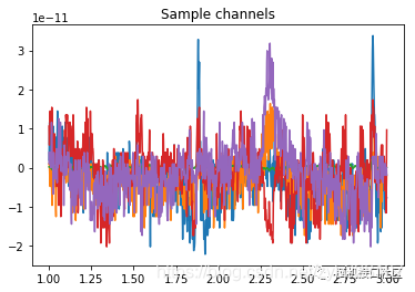
"""
绘制各通道的功率谱密度
"""
raw.plot_psd()
plt.show()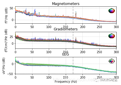
"""
绘制SSP矢量图
"""
raw.plot_projs_topomap()
plt.show()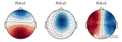
"""
绘制通道频谱图作为topography
"""
raw.plot_psd_topo()
plt.show()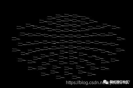
"""
绘制电极位置
"""
raw.plot_sensors()
plt.show()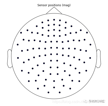
MNE 从头创建Raw对象
在实际过程中,有时需要从头构建数据来创建Raw对象。
方式:通过mne.io.RawArray类来手动创建Raw
注:使用mne.io.RawArray创建Raw对象时,其构造函数只接受矩阵和info对象。
数据对应的单位:
V: eeg, eog, seeg, emg, ecg, bio, ecog
T: mag
T/m: grad
M: hbo, hbr
Am: dipole
AU: misc
构建一个Raw对象时,需要准备两种数据,一种是data数据,一种是Info数据,
data数据是一个二维数据,形状为(n_channels,n_times)
案例1
import mne
import numpy as np
import matplotlib.pyplot as plt

"""
生成一个大小为5x1000的二维随机数据
其中5代表5个通道,1000代表times
"""
data = np.random.randn(5, 1000)

"""
创建info结构,
内容包括:通道名称和通道类型
设置采样频率为:sfreq=100
"""
info = mne.create_info(
    ch_names=['MEG1', 'MEG2', 'EEG1', 'EEG2', 'EOG'],
    ch_types=['grad', 'grad', 'eeg', 'eeg', 'eog'],
    sfreq=100
)
"""
利用mne.io.RawArray类创建Raw对象
"""
custom_raw = mne.io.RawArray(data, info)
print(custom_raw)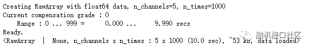
从上面打印的信息可以看出
raw对象中n_channels=5, n_times=1000
"""
对图形进行缩放

对于实际的EEG / MEG数据,应使用不同的比例因子。
对通道eeg、grad,eog的数据进行2倍缩小
"""
scalings = {'eeg': 2, 'grad': 2,'eog':2}
custom_raw.plot(n_channels=5,
                scalings=scalings,
                title='Data from arrays',
         show=True, block=True)

plt.show()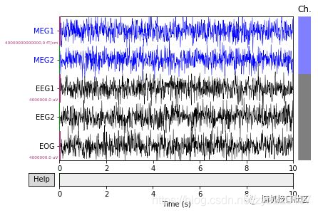
案例2
import numpy as np
import neo
import mne
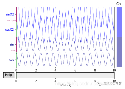
import matplotlib.pyplot as plt构建正余弦数据模拟mag,grad信号
其中采样频率为1000Hz,时间为0到10s.
# 创建任意数据
sfreq = 1000  # 采样频率
times = np.arange(0, 10, 0.001)  # Use 10000 samples (10s)

sin = np.sin(times * 10)  # 乘以 10 缩短周期
cos = np.cos(times * 10)
sinX2 = sin * 2
cosX2 = cos * 2

# 数组大小为 4 X 10000.
data = np.array([sin, cos, sinX2, cosX2])

# 定义 channel types and names.
ch_types = ['mag', 'mag', 'grad', 'grad']
ch_names = ['sin', 'cos', 'sinX2', 'cosX2']
创建info对象
"""
创建info对象
"""
info = mne.create_info(ch_names=ch_names,
                       sfreq=sfreq,
                       ch_types=ch_types)
利用mne.io.RawArray创建raw对象
"""
利用mne.io.RawArray创建raw对象
"""
raw = mne.io.RawArray(data, info)

"""
对图形进行缩放

对于实际的EEG / MEG数据,应使用不同的比例因子。

对通道mag的数据进行2倍缩小,对grad的数据进行1.7倍缩小
"""
scalings = {'mag': 2, 'grad':1.7}

raw.plot(n_channels=4, scalings=scalings, title='Data from arrays',
         show=True, block=True)

"""
可以采用自动缩放比例

只要设置scalings='auto'即可
"""
scalings = 'auto'
raw.plot(n_channels=4, scalings=scalings,
         title='Auto-scaled Data from arrays',
         show=True, block=True)
plt.show()
本文章由脑机学习者Rose笔记分享,QQ交流群:903290195
更多分享,请关注公众号