- 1. A Short-Sighted Algorithm
- 2. Guarantee the Solution to Be Global Optimal
- 3. Batch Gradient Descent for Linear Regression - Steps to Solve a Greedy Task
- 4. General Structure of Greedy Algorithm
- 5. Pair Work
1. A Short-Sighted Algorithm
Greedy algorithm is another method of finding out the optimal solution, or the nearly optimal one of a task. Unlike DP, however, the Greedy algorithm may not always be able to find out the GLOBAL optimum, sometimes it will give you a LOCAL optimum instead.
The intuition of the algorithm is that, it always chooses the optimal solution for the current step, so that the overall solution may be also optimal. Suppose we want to get ¥6 now and we have some ¥1, ¥2, ¥5. What we will commonly do is first find a ¥5 and then a ¥1. Notice that we first find the greatest value that is smaller than or equal to the amount we want to get, ¥5 here which is smaller than ¥6. Then the new amount we want to get is ¥1. Since ¥1 is smaller than or equal to ¥1, we take the ¥1. Both ¥5 and ¥1 here are the optimal solution for the corresponding amount (the corresponding task).
When the values are ¥1, ¥3, ¥4, however, the greedy algorithm can not permit to find out the optimal solution. When the greedy algorithm is applied, the solution will be {4, 1, 1}. However, the optimal solution for the case here is actually {3, 3}. It's a situation that the greedy algorithm eventually finds out a local optimum instead of a global one.
One more difference between DP and the greedy algorithm is that the overall solution to DP relies on the solutions to its sub-tasks, while the greedy algorithm makes decisions without considering solutions to any sub-tasks.
2. Guarantee the Solution to Be Global Optimal
The greedy algorithm cannot always find out the optimal solution to a task. However, it a task has two properties:
- Greedy Choice Property
- Optimal Substructure
the optimal solution can always be found out with the greedy algorithm. They can be used to judge if the optimal solution to a task can be found out with the greedy algorithm.
2.1. Greedy Choice Property
The greedy choice property means that each choice (each solution to the sub-tasks) are greedy choices, that is, the best choices for the corresponding sub-tasks.
Pruning is a common way to find out if a task has the greedy choice property. Here's what it does:
- Assume that we now have an optimal solution which is NOT calculated by the greedy choice.
- Replace the choice with the greedy choice.
- Prove that the replaced solution is better, or at least as good as the original solution.
2.1.1. Greedy Choice Property in the Filling up Problem / 汽车加油问题的贪心选择性质
Here's a concrete example illustrating the way to prove if a task has the greedy choice property. The original question is below and only the proof of the property is given here.
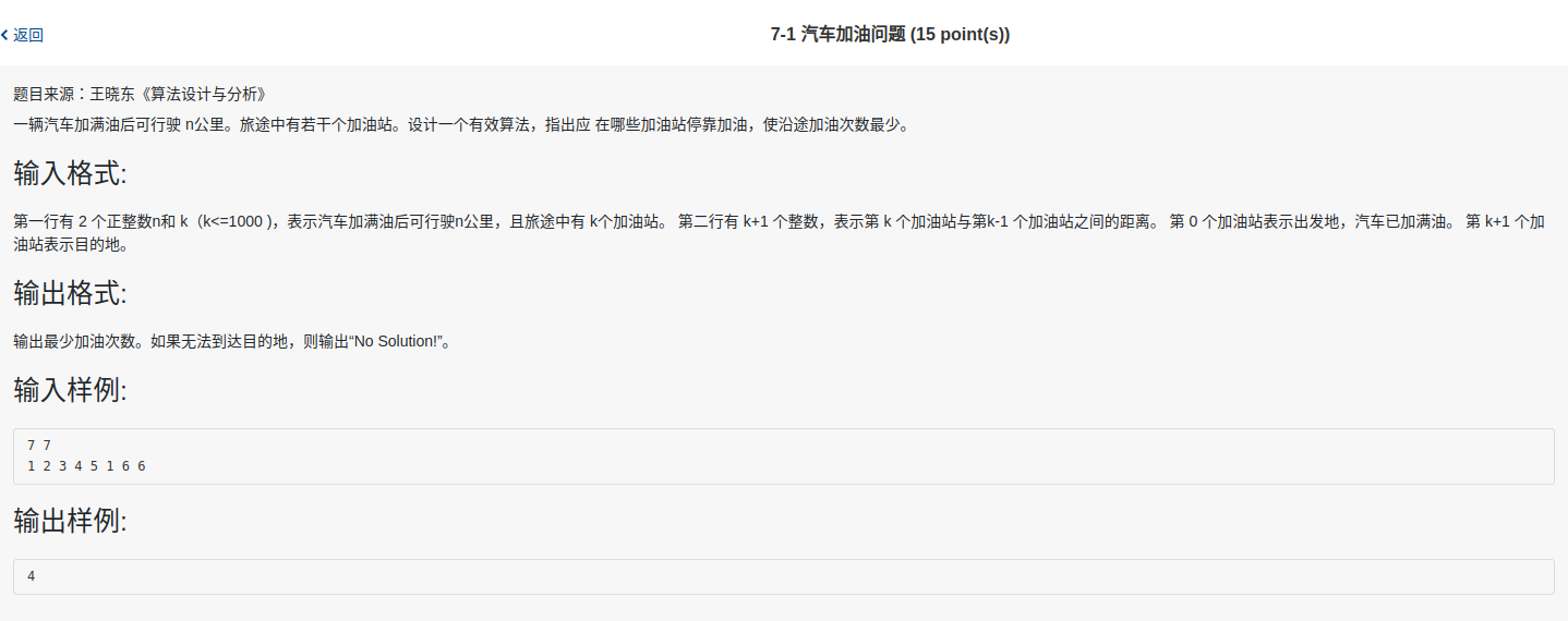
The goal of the task is to find out the least times for filling up. And it's not hard to think of the greedy choice for the task: the gasoline stand chosen every time is the stand that when the car reaches, the remaining gasoline volume should be the least. And here's the proof.
Suppose we got an optimal solution with choosing a stand which is NOT the optimal one. In other words, we chose a stand that there is at least one stand that when the car reaches, the remaining gasoline volume of the car is less than when the car reaches the stand we've chosen.
And we now replace the stand we've chosen with the greedy choice. The greedy choice here must be a stand which is after the stand we've chosen, so that the remaining gasoline volume is less when the car reaches the greedily chosen stand.
Since the greedy choice is farther, the car can run farther without the need to fill up. And therefore the times of filling up decreases. The solution gets better.
Thus the task here has the greedy choice property.
2.2. Optimal Substructure
If the solution to a task can be found with the greedy algorithm, it has an optimal substructure. The optimal substructure property is the same as that in DP.
I provided a way to prove if a task has an optimal substructure in the summary of chapter 3
3. Batch Gradient Descent for Linear Regression - Steps to Solve a Greedy Task
Gradient descent is a greedy algorithm and can be used as the optimization algorithm for linear regression.
Detailed discussions about gradient descent can be accessed from here. I'm going to discuss GD as a greedy algorithm here and will omit details of linear regression. Details of linear regression can be referenced in books talking about machine learning.
For simplicity I'm going to discuss the gradient descent algorithm with a pretty simple linear regression model:
\[\boldsymbol {\hat y} = \boldsymbol w \boldsymbol x + b\]
where \(\boldsymbol x\) is the vector of training set, \(\boldsymbol {\hat y}\) is the predicted vector, \(\boldsymbol w\) is the parameter vector, and \(b\) is a number.
And its cost function is:
\[J(\boldsymbol w, b) = \sum^m_{i = 1}(\hat y - y)^2\]
Let's optimize the function with Batch Gradient Descent, which is a type of GD, manipulating all training instances in every loop. The formula of BGD is:
\[\boldsymbol \theta := \boldsymbol \theta - \eta \Delta \boldsymbol \theta; \\ \Delta \boldsymbol \theta = \frac{\partial}{\partial \boldsymbol \theta}J\]
where \(\eta > 0\) is the learning rate, just treat it as a constant here. \(\theta\) is the parameter to be calculated and \(J\) is the cost function to be optimized.
For linear regression, BGD can find out the optimal solution (the optimal \(\theta\)) to minimize the cost function. It means BGD for linear regression satisfies the two properties of the greedy algorithm. Let's prove it below.
3.1. Two Properties
3.1.1. Greedy Choice Property
Our task is to minimize the cost function \(J\) as fast as we can, so \(\Delta \boldsymbol \theta\) should be the greatest for every loop. According to maths the greatest \(\Delta \boldsymbol \theta\) here is the opposite number of gradient of \(J\), as the gradient of a function is the direction where the value of the function increases the most quickly. Thus the greedy choice of the task here is the gradient of \(J\).
Let's use the strategy discussed above to prove the property.
Suppose we now got an optimal solution without the greedy choice. In the task here we get a \(\Delta \boldsymbol \theta\) which is not the gradient of \(J\). And let's say the formula of GD now is
\[\boldsymbol \theta^{'} := \boldsymbol \theta - \eta \Delta \boldsymbol \theta\]
Then we replace \(\Delta \boldsymbol \theta\) here with the gradient of \(J\), which is \(\frac{\partial}{\partial \boldsymbol \theta}J\), and the formula now is
\[\boldsymbol \theta := \boldsymbol \theta - \eta \frac{\partial}{\partial \boldsymbol \theta}J\]
and since
\[ \begin{aligned} \frac{\partial}{\partial \boldsymbol \theta}J &> \Delta \boldsymbol \theta \\ -\frac{\partial}{\partial \boldsymbol \theta}J &< -\Delta \boldsymbol \theta \\ -\eta \frac{\partial}{\partial \boldsymbol \theta}J &< -\eta \Delta \boldsymbol \theta \\ \boldsymbol \theta -\eta \frac{\partial}{\partial \boldsymbol \theta}J &< \boldsymbol \theta -\eta \Delta \boldsymbol \theta \\ \boldsymbol \theta &< \boldsymbol {\theta^{'}} \\ \end{aligned} \]
Thus the solution with the greedy choice is better than the one without the greedy choice, and we now have confidence to say BGD for linear regression satisfies the greedy choice property.
3.1.2. Optimal Substructure
Let's say the collection of the calculated \(\theta\)s is \(\{\boldsymbol \theta^{(1)}, \boldsymbol \theta^{(2)},\; ..., \boldsymbol\theta^{(n - 1)}, \boldsymbol \theta^{(n)}\}\). And the corresponding cost function for \(\boldsymbol \theta^{(n)}\) is \(J(\boldsymbol \theta^{(n)})\).
The substructure for the task here is \(\{\boldsymbol \theta^{(1)}, \boldsymbol \theta^{(2)},\; ..., \boldsymbol\theta^{(n - 1)}\}\), and the corresponding cost function for \(\boldsymbol \theta^{(n - 1)}\) is \(J(\boldsymbol \theta^{(n - 1)})\).
Assume that the substructure here is not the optimal one, and the optimal one is \(\{\boldsymbol \theta^{(1^{'})}, \boldsymbol \theta^{(2^{'})},\; ..., \boldsymbol\theta^{((n - 1)^{'})}\}\). So
\[J(\boldsymbol \theta^{((n - 1)^{'})}) < J(\boldsymbol \theta^{(n - 1)})\]
According to mathematical derivation,
\[J(\boldsymbol \theta^{(n)^{'})}) < J(\boldsymbol \theta^{n})\]
But in reality
\[J(\boldsymbol \theta^{(n)^{'})}) > J(\boldsymbol \theta^{n})\]
Thus it's contradictory and the assumption is not tenable.
3.2. Implementation
The discussion above shows BGD for linear regression can help find the GLOBAL OPTIMA. And we have formulas for updating \(\boldsymbol w\) and \(b\).
\[ \begin{aligned} \boldsymbol w &:= \boldsymbol w - \eta \frac{\partial}{\partial \boldsymbol w}J(\boldsymbol w, b) \\ b &:= b - \eta \frac{\partial}{\partial b}J(\boldsymbol w, b) \end{aligned} \]
The formula is for a single training example. We can use a vectorized form of the training set to process all instances together in a loop.
eta = 0.1  # learning rate
n_iterations = 1000  # number of iterations

m = 100  # data size

theta = np.random.randn(2, 1)  # random init

# BGD
for iteration in range(n_iterations):
  W -= eta * gradient(J, W)  # update W
  b -= eta * gradient(J, b)  # update b

  J = J(W, b)
gradient(J, x) calculates \(\frac{\partial}{\partial x}J\) and J(W, b) calculates the value of the cost function \(J\).
Situations when Local Optima Will Be Found
BGD can be applied to linear regression to find the GLOBAL OPTIMA because:
- The cost function of linear regression is a convex function, which means that if you pick any two points on the curve, the line segment joining them never crosses the curve. This implies that there are no local minima, just one global minimum.
- It is a continuous function with a slope that never changes abruptly.
These two facts have a great consequence: Gradient Descent is guaranteed to approach arbitrarily close the global minimum (if you wait long enough and if the learning rate is not too high).
But if a cost function doesn't satisfy the properties above, BGD may not able to find out its global optima, but LOCAL OPTIMA instead.

Notice the left part of the function. There are local optima. BGD may not find the local optimum if \(\theta\) is initialized with an improper value, or the learning rate is set too small.
4. General Structure of Greedy Algorithm
The greedy algorithm gradually finds the optimal solution(the greedy choice) to each sub-task. Solutions can be put in a set. And the process of searching for optimal solutions can be wrapped in a for loop or a while loop. There may be conditions or functions determining if the current solution is the optimal one, that is, the greedy choice. And there may be a function judging if the constraint of the task is satisfied after adding the current optimal solution to the solution set. Sometimes such functionality is implemented by the sort function.
while (the solution of the task has not yet been constructed) {
  find out the greedy choice

  if (the constraint is satisfied) {
    add the solution to the solution set
  } else {
    ...
  }
}
Pair Work
The first question was not hard and we finished it quickly. The second question, however, was not as easy as we thought and we got stuck in it. We tried pretty lots of methods and finally with the help of the Internet we finished it. The solution to the third question was not hard, which was similar to that of the Huffman algorithm, but it was a pity that I didn't have enough time to finish it.