电影的影评一般分为正面(positive)或负面(nagetive)两类。这是一个二元(binary)或者二分类问题,一种重要且应用广泛的机器学习问题。
我们将使用来源于网络电影数据库(Internet Movie Database)的 IMDB 数据集(IMDB dataset),其包含 50,000 条影评文本。从该数据集切割出的25,000条评论用作训练,另外 25,000 条用作测试。训练集与测试集是平衡的(balanced),意味着它们包含相等数量的积极和消极评论。
本文的代码来自tensorflow教程官网
数据下载
和之前项目一样,首先配置环境参数 具体代码如下:
from __future__ import absolute_import, division, print_function, unicode_literals#该行要放在第一行位置
import warnings#忽略系统警告提示
warnings.filterwarnings('ignore')
import tensorflow as tf
from tensorflow import keras

import numpy as np
print(tf.__version__)
2.0.0
基本配置设定完毕后,可以下载数据集。IMDB 数据集已经打包在 Tensorflow 中。该数据集已经经过预处理,评论(单词序列)已经被转换为整数序列,其中每个整数表示字典中的特定单词。具体代码如下:
imdb = keras.datasets.imdb
(train_data, train_labels), (test_data, test_labels) = imdb.load_data(num_words=10000)#参数 num_words=10000 保留了训练数据中最常出现的 10,000 个单词。为了保持数据规模的可管理性,低频词将被丢弃。
参数 num_words=10000 保留了训练数据中最常出现的 10,000 个单词,注意10000是指常用单词数量,并非下载的样本数量。为了保持数据规模的可管理性,低频词将被丢弃。
这里如果您已经下载过该数据集,则会直接从缓存中复制。
了解数据
让我们花一点时间来了解数据格式。该数据集是经过预处理的:每个样本都是一个表示影评中词汇的整数数组。每个标签都是一个值为 0 或 1 的整数值,其中 0 代表消极评论,1 代表积极评论。
print('Training entries: {}, labels: {}'.format(len(train_data), len(train_labels)))Training entries: 25000, labels: 25000#25000个样本和25000个标签
评论文本被转换为整数值,其中每个整数代表词典中的一个单词。(注意:这里我本来以为每个数字代表的是26个字母中的一个。。。这里就是字面意思,一个单词,具体我会在下面详细说明)我们以第一条评论为例:
print(train_data[0]) #这里一定要注意,每个数字代表的是单词,不是字母。[1, 14, 22, 16, 43, 530, 973, 1622, 1385, 65, 458, 4468, 66, 3941, 4, 173, 36, 256, 5, 25, 100, 43, 838, 112, 50, 670, 2, 9, 35, 480, 284, 5, 150, 4, 172, 112, 167, 2, 336, 385, 39, 4, 172, 4536, 1111, 17, 546, 38, 13, 447, 4, 192, 50, 16, 6, 147, 2025, 19, 14, 22, 4, 1920, 4613, 469, 4, 22, 71, 87, 12, 16, 43, 530, 38, 76, 15, 13, 1247, 4, 22, 17, 515, 17, 12, 16, 626, 18, 2, 5, 62, 386, 12, 8, 316, 8, 106, 5, 4, 2223, 5244, 16, 480, 66, 3785, 33, 4, 130, 12, 16, 38, 619, 5, 25, 124, 51, 36, 135, 48, 25, 1415, 33, 6, 22, 12, 215, 28, 77, 52, 5, 14, 407, 16, 82, 2, 8, 4, 107, 117, 5952, 15, 256, 4, 2, 7, 3766, 5, 723, 36, 71, 43, 530, 476, 26, 400, 317, 46, 7, 4, 2, 1029, 13, 104, 88, 4, 381, 15, 297, 98, 32, 2071, 56, 26, 141, 6, 194, 7486, 18, 4, 226, 22, 21, 134, 476, 26, 480, 5, 144, 30, 5535, 18, 51, 36, 28, 224, 92, 25, 104, 4, 226, 65, 16, 38, 1334, 88, 12, 16, 283, 5, 16, 4472, 113, 103, 32, 15, 16, 5345, 19, 178, 32]
电影评论可能具有不同的长度。以下代码显示了第一条和第二条评论的中单词数量。由于神经网络的输入必须是统一的长度,我们稍后需要解决这个问题。
len(train_data[0]), len(train_data[1])(218, 189)
将整数转换回单词
对于上面一串数字代表的具体含义,大家肯定很好奇。了解如何将整数转换回文本对您可能是有帮助的。这里我们将创建一个辅助函数来查询一个包含了整数到字符串映射的字典对象:
#一个映射单词到整数索引的词典
word_index = imdb.get_word_index()#建立词典索引
#保留第一个索引
word_index = {k:(v+3) for k,v in word_index.items()}
word_index["<PAD>"] = 0#这里0代表<PAD>
word_index["<START>"] = 1#这里1代表<START>
word_index["<UNK>"] = 2#这里2代表<UNK>(unknown)
word_index["<UNUSED>"] = 3#这里3代表<UNUSED>

reverse_word_index = dict([(value, key) for (key, value) in word_index.items()])
def decode_review(text):
    return ' '.join([reverse_word_index.get(i, '?') for i in text])
字典建立完毕后,我们可以使用 decode_review 函数来显示首条评论的文本:
decode_review(train_data[0])"<START> this film was just brilliant casting location scenery story direction everyone's really suited the part they played and you could just imagine being there robert <UNK> is an amazing actor and now the same being director <UNK> father came from the same scottish island as myself so i loved the fact there was a real connection with this film the witty remarks throughout the film were great it was just brilliant so much that i bought the film as soon as it was released for <UNK> and would recommend it to everyone to watch and the fly fishing was amazing really cried at the end it was so sad and you know what they say if you cry at a film it must have been good and this definitely was also <UNK> to the two little boy's that played the <UNK> of norman and paul they were just brilliant children are often left out of the <UNK> list i think because the stars that play them all grown up are such a big profile for the whole film but these children are amazing and should be praised for what they have done don't you think the whole story was so lovely because it was true and was someone's life after all that was shared with us all"
数据处理
准备数据
由于神经网络的输入必须是张量形式,因此影评需要首先转换为张量,然后才可以进行学习,转换的方式有两种:
1 将数组转换为表示单词出现与否的由 0 和 1 组成的向量,类似于 one-hot 编码。例如,序列[3, 5]将转换为一个 10,000 维的向量,该向量除了索引为 3 和 5 的位置是 1 以外,其他都为 0。然后,将其作为网络的首层——一个可以处理浮点型向量数据的稠密层。不过,这种方法需要大量的内存,需要一个大小为 num_words * num_reviews 的矩阵。
2 我们可以填充数组来保证输入数据具有相同的长度,然后创建一个大小为 max_length * num_reviews 的整型张量。我们可以使用能够处理此形状数据的嵌入层作为网络中的第一层。
在本示例中,我们将使用第二种方法。
由于电影评论长度必须相同,我们将使用 pad_sequences 函数来使长度标准化:
#训练数据长度设置为256
train_data = keras.preprocessing.sequence.pad_sequences(train_data,
                                                        value=word_index["<PAD>"],
                                                        padding='post',
                                                         maxlen=256)
#测试数据长度设置为256
test_data = keras.preprocessing.sequence.pad_sequences(test_data,
                                                       value=word_index["<PAD>"],
                                                       padding='post',
                                                        maxlen=256)
现在让我们看下样本的长度:
len(train_data[0]), len(train_data[1])
(256, 256)
我们再检查一下首条评论(当前已经填充)
print(train_data[0])[ 1 14 22 16 43 530 973 1622 1385 65 458 4468 66 3941
4 173 36 256 5 25 100 43 838 112 50 670 2 9
35 480 284 5 150 4 172 112 167 2 336 385 39 4
172 4536 1111 17 546 38 13 447 4 192 50 16 6 147
2025 19 14 22 4 1920 4613 469 4 22 71 87 12 16
43 530 38 76 15 13 1247 4 22 17 515 17 12 16
626 18 2 5 62 386 12 8 316 8 106 5 4 2223
5244 16 480 66 3785 33 4 130 12 16 38 619 5 25
124 51 36 135 48 25 1415 33 6 22 12 215 28 77
52 5 14 407 16 82 2 8 4 107 117 5952 15 256
4 2 7 3766 5 723 36 71 43 530 476 26 400 317
46 7 4 2 1029 13 104 88 4 381 15 297 98 32
2071 56 26 141 6 194 7486 18 4 226 22 21 134 476
26 480 5 144 30 5535 18 51 36 28 224 92 25 104
4 226 65 16 38 1334 88 12 16 283 5 16 4472 113
103 32 15 16 5345 19 178 32 0 0 0 0 0 0
0 0 0 0 0 0 0 0 0 0 0 0 0 0
0 0 0 0 0 0 0 0 0 0 0 0 0 0
0 0 0 0]
可以看到现在数据长度均为256。
模型搭建
模型网络架构
接下来进行模型的搭建,神经网络由堆叠的层来构建,这需要从两个主要方面来进行体系结构决策:
模型里有多少层?
每个层里有多少隐层单元(hidden units)?
在此样本中,输入数据包含一个单词索引的数组。要预测的标签为 0 或 1。让我们来为该问题构建一个模型,首先我们利用keras.Sequential进行层的序列化添加,具体代码如下:
# 输入形状是用于电影评论的词汇数目(10,000 词)
vocab_size = 10000
model = keras.sequential()#搭建层
model.add(keras.layers.Embedding(vocab_size, 16))#embedding 是一个将单词向量化的函数,嵌入(embeddings)输出的形状都是:(num_examples, embedding_dimension)
model.add(keras.layers.GloabAveragePooling1D())#添加全局平均池化层
model.add(keras.layers.Dense(16, activation = 'relu'))
model.add(keras.layers.Dense(1, activation = 'sigmoid'))

model.summary()
Model: "sequential"
_________________________________________________________________
Layer (type) Output Shape Param #
=================================================================
embedding (Embedding) (None, None, 16) 160000
_________________________________________________________________
global_average_pooling1d (Gl (None, 16) 0
_________________________________________________________________
dense (Dense) (None, 16) 272
_________________________________________________________________
dense_1 (Dense) (None, 1) 17
=================================================================
Total params: 160,289
Trainable params: 160,289
Non-trainable params: 0
层按顺序堆叠以构建分类器:
第一层是嵌入(Embedding)层。该层采用整数编码的词汇表,并查找每个词索引的嵌入向量(embedding vector)。这些向量是通过模型训练学习到的。向量向输出数组增加了一个维度。得到的维度为:(batch, sequence, embedding)。
embedding 是一个将单词向量化的函数,嵌入(embeddings)输出的形状都是:(num_examples, embedding_dimension)
接下来,GlobalAveragePooling1D 将通过对序列维度求平均值来为每个样本返回一个定长输出向量。这允许模型以尽可能最简单的方式处理变长输入。
该定长输出向量通过一个有 16 个隐层单元的全连接(Dense)层传输。
最后一层与单个输出结点密集连接。使用 Sigmoid 激活函数,其函数值为介于 0 与 1 之间的浮点数,表示概率或置信度。
模型编译
model.compile(optimize = 'adam',
              loss = 'binary_crossentropy',
              metrics = ['accuracy'])
模型评估
验证模型
x_val = train_data[:10000]#取训练数据集前10000个进行训练和验证
partial_x_train = train_data[10000:]
y_val = train_labels[:10000]#同理取前10000个标签
partial_y_train = train_labels[10000:]
模型训练
#以 512 个样本的 mini-batch 大小迭代 40 个 epoch 来训练模型。这是指对 x_train 和 y_train 张量中所有样本的的 40 次迭代。在训练过程中,监测来自验证集的 10,000 个样本上的损失值(loss)和准确率(accuracy):
history = model.fit(partial_x_train,
                    partial_y_train,
                    epochs=40,
                    batch_size=512,
                    validation_data=(x_val, y_val),
                    verbose=1)
Train on 15000 samples, validate on 10000 samples
Epoch 1/40
15000/15000 [==============================] - 1s 88us/sample - loss: 0.6924 - accuracy: 0.6045 - val_loss: 0.6910 - val_accuracy: 0.6819
Epoch 2/40
15000/15000 [==============================] - 0s 22us/sample - loss: 0.6885 - accuracy: 0.6392 - val_loss: 0.6856 - val_accuracy: 0.7129
Epoch 3/40
15000/15000 [==============================] - 0s 22us/sample - loss: 0.6798 - accuracy: 0.7371 - val_loss: 0.6747 - val_accuracy: 0.7141
Epoch 4/40
15000/15000 [==============================] - 0s 22us/sample - loss: 0.6629 - accuracy: 0.7648 - val_loss: 0.6539 - val_accuracy: 0.7597
Epoch 5/40
15000/15000 [==============================] - 0s 21us/sample - loss: 0.6356 - accuracy: 0.7860 - val_loss: 0.6239 - val_accuracy: 0.7783
Epoch 6/40
15000/15000 [==============================] - 0s 22us/sample - loss: 0.5975 - accuracy: 0.8036 - val_loss: 0.5849 - val_accuracy: 0.7931
Epoch 7/40
15000/15000 [==============================] - 0s 22us/sample - loss: 0.5525 - accuracy: 0.8195 - val_loss: 0.5421 - val_accuracy: 0.8076
Epoch 8/40
15000/15000 [==============================] - 0s 22us/sample - loss: 0.5025 - accuracy: 0.8357 - val_loss: 0.4961 - val_accuracy: 0.8245
Epoch 9/40
15000/15000 [==============================] - 0s 22us/sample - loss: 0.4541 - accuracy: 0.8537 - val_loss: 0.4555 - val_accuracy: 0.8392
Epoch 10/40
15000/15000 [==============================] - 0s 22us/sample - loss: 0.4114 - accuracy: 0.8672 - val_loss: 0.4211 - val_accuracy: 0.8469
Epoch 11/40
15000/15000 [==============================] - 0s 22us/sample - loss: 0.3753 - accuracy: 0.8775 - val_loss: 0.3938 - val_accuracy: 0.8531
Epoch 12/40
15000/15000 [==============================] - 0s 22us/sample - loss: 0.3451 - accuracy: 0.8859 - val_loss: 0.3713 - val_accuracy: 0.8600
Epoch 13/40
15000/15000 [==============================] - 0s 21us/sample - loss: 0.3201 - accuracy: 0.8924 - val_loss: 0.3540 - val_accuracy: 0.8665
Epoch 14/40
15000/15000 [==============================] - 0s 22us/sample - loss: 0.2990 - accuracy: 0.8983 - val_loss: 0.3397 - val_accuracy: 0.8712
Epoch 15/40
15000/15000 [==============================] - 0s 23us/sample - loss: 0.2809 - accuracy: 0.9037 - val_loss: 0.3290 - val_accuracy: 0.8735
Epoch 16/40
15000/15000 [==============================] - 0s 22us/sample - loss: 0.2649 - accuracy: 0.9095 - val_loss: 0.3197 - val_accuracy: 0.8766
Epoch 17/40
15000/15000 [==============================] - 0s 22us/sample - loss: 0.2508 - accuracy: 0.9131 - val_loss: 0.3121 - val_accuracy: 0.8792
Epoch 18/40
15000/15000 [==============================] - 0s 22us/sample - loss: 0.2379 - accuracy: 0.9183 - val_loss: 0.3063 - val_accuracy: 0.8797
Epoch 19/40
15000/15000 [==============================] - 0s 22us/sample - loss: 0.2262 - accuracy: 0.9216 - val_loss: 0.3013 - val_accuracy: 0.8806
Epoch 20/40
15000/15000 [==============================] - 0s 21us/sample - loss: 0.2156 - accuracy: 0.9261 - val_loss: 0.2972 - val_accuracy: 0.8828
Epoch 21/40
15000/15000 [==============================] - 0s 22us/sample - loss: 0.2061 - accuracy: 0.9292 - val_loss: 0.2939 - val_accuracy: 0.8827
Epoch 22/40
15000/15000 [==============================] - 0s 22us/sample - loss: 0.1966 - accuracy: 0.9329 - val_loss: 0.2918 - val_accuracy: 0.8833
Epoch 23/40
15000/15000 [==============================] - 0s 21us/sample - loss: 0.1881 - accuracy: 0.9368 - val_loss: 0.2892 - val_accuracy: 0.8837
Epoch 24/40
15000/15000 [==============================] - 0s 22us/sample - loss: 0.1802 - accuracy: 0.9408 - val_loss: 0.2884 - val_accuracy: 0.8841
Epoch 25/40
15000/15000 [==============================] - 0s 21us/sample - loss: 0.1725 - accuracy: 0.9436 - val_loss: 0.2871 - val_accuracy: 0.8845
Epoch 26/40
15000/15000 [==============================] - 0s 22us/sample - loss: 0.1656 - accuracy: 0.9468 - val_loss: 0.2863 - val_accuracy: 0.8856
Epoch 27/40
15000/15000 [==============================] - 0s 22us/sample - loss: 0.1592 - accuracy: 0.9494 - val_loss: 0.2863 - val_accuracy: 0.8862
Epoch 28/40
15000/15000 [==============================] - 0s 21us/sample - loss: 0.1529 - accuracy: 0.9516 - val_loss: 0.2868 - val_accuracy: 0.8851
Epoch 29/40
15000/15000 [==============================] - 0s 21us/sample - loss: 0.1465 - accuracy: 0.9555 - val_loss: 0.2871 - val_accuracy: 0.8860
Epoch 30/40
15000/15000 [==============================] - 0s 22us/sample - loss: 0.1410 - accuracy: 0.9568 - val_loss: 0.2882 - val_accuracy: 0.8858
Epoch 31/40
15000/15000 [==============================] - 0s 22us/sample - loss: 0.1354 - accuracy: 0.9591 - val_loss: 0.2896 - val_accuracy: 0.8858
Epoch 32/40
15000/15000 [==============================] - 0s 24us/sample - loss: 0.1303 - accuracy: 0.9618 - val_loss: 0.2906 - val_accuracy: 0.8865
Epoch 33/40
15000/15000 [==============================] - 0s 24us/sample - loss: 0.1251 - accuracy: 0.9639 - val_loss: 0.2923 - val_accuracy: 0.8858
Epoch 34/40
15000/15000 [==============================] - 0s 23us/sample - loss: 0.1206 - accuracy: 0.9658 - val_loss: 0.2941 - val_accuracy: 0.8858
Epoch 35/40
15000/15000 [==============================] - 0s 23us/sample - loss: 0.1164 - accuracy: 0.9668 - val_loss: 0.2972 - val_accuracy: 0.8849
Epoch 36/40
15000/15000 [==============================] - 0s 24us/sample - loss: 0.1116 - accuracy: 0.9683 - val_loss: 0.2992 - val_accuracy: 0.8845
Epoch 37/40
15000/15000 [==============================] - 0s 23us/sample - loss: 0.1075 - accuracy: 0.9709 - val_loss: 0.3010 - val_accuracy: 0.8842
Epoch 38/40
15000/15000 [==============================] - 0s 24us/sample - loss: 0.1036 - accuracy: 0.9715 - val_loss: 0.3067 - val_accuracy: 0.8807
Epoch 39/40
15000/15000 [==============================] - 0s 24us/sample - loss: 0.0996 - accuracy: 0.9724 - val_loss: 0.3068 - val_accuracy: 0.8830
Epoch 40/40
15000/15000 [==============================] - 0s 24us/sample - loss: 0.0956 - accuracy: 0.9749 - val_loss: 0.3109 - val_accuracy: 0.8823
评估模型
我们来看一下模型的性能如何。将返回两个值。损失值(loss)(一个表示误差的数字,值越低越好)与准确率(accuracy)。
results = model.evaluate(test_data,  test_labels, verbose=2)
print(results)
25000/1 - 2s - loss: 0.3454 - accuracy: 0.8732
[0.32927662477493286, 0.8732]
这种十分朴素的方法得到了约 87% 的准确率(accuracy)。若采用更好的方法,模型的准确率应当接近 95%。更优化的方法我会另行介绍。
创建一个准确率(accuracy)和损失值(loss)随时间变化的图表
model.fit() 返回一个 History 对象,该对象包含一个字典,其中包含训练阶段所发生的一切事件:
history_dict = history.history
history_dict.keys()
dict_keys(['loss', 'accuracy', 'val_loss', 'val_accuracy'])#注意这里返回的值,这里需要与下面的代码完全对应否则运算报错。
有四个条目:在训练和验证期间,每个条目对应一个监控指标。我们可以使用这些条目来绘制训练与验证过程的损失值(loss)和准确率(accuracy),以便进行比较。根据原教程的代码,在tensorflow1.1.14版本会有报错现象发生,下面我会详细指出。
import matplotlib.pyplot as plt
acc = history_dict['accuracy']#这里应改为acc
val_acc = history_dict['val_accuracy']#这里应该改为val_acc
loss = history_dict['loss']
val_loss = history_dict['val_loss']

epochs = range(1, len(acc) + 1)
# “bo”代表 "蓝点"
plt.plot(epochs, loss, 'bo', label='Training loss')
# b代表“蓝色实线”
plt.plot(epochs, val_loss, 'b', label='Validation loss')
plt.title('Training and validation loss')
plt.xlabel('Epochs')
plt.ylabel('Loss')
plt.legend()

plt.show()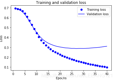
plt.clf()   # 清除数字
plt.plot(epochs, acc, 'bo', label='Training acc')
plt.plot(epochs, val_acc, 'b', label='Validation acc')
plt.title('Training and validation accuracy')
plt.xlabel('Epochs')
plt.ylabel('Accuracy')
plt.legend()
plt.show()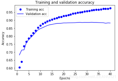
在该图中,点代表训练损失值(loss)与准确率(accuracy),实线代表验证损失值(loss)与准确率(accuracy)。
注意训练损失值随每一个 epoch 下降而训练准确率(accuracy)随每一个 epoch 上升。这在使用梯度下降优化时是可预期的——理应在每次迭代中最小化期望值。
验证过程的损失值(loss)与准确率(accuracy)的情况却并非如此——它们似乎在 20 个 epoch 后达到峰值。这是过拟合的一个实例:模型在训练数据上的表现比在以前从未见过的数据上的表现要更好。在此之后,模型过度优化并学习特定于训练数据的表示,而不能够泛化到测试数据。
对于这种特殊情况,我们可以通过在 20 个左右的 epoch 后停止训练来避免过拟合。
总结
对于keras深度学习的网络架构而言,主要分为如下几个步骤:
1,载入数据
2,预处理数据
3,定义模型
4,编译模型
5,训练模型
6,评估模型
7,预测
8,保存模型
对于如何保存模型,如何将训练好的模型直接拿来对我们自己的数据进行预测,我会在其他版块加以说明。