机器学习 | 调参 Part2

关于调参，前面已经完成了一篇，重点介绍了网格搜索和随机搜索，详情见：机器学习 | 调参 Part1，本篇博客将重点介绍下贝叶斯调参！

1 贝叶斯调参思想

话说这个贝叶斯是个什么鬼，真的有点绕啊！看几个资料看的好久，但还是有点云里雾里，所以今天小编和大家分享一下自己的学习体会，如果有不对的，还请大家多多担待！

首先来聊一聊什么是贝叶斯调参？它和前两种调参方式有什么区别呢？又有什么优势呢？不然为啥要花大力气看它呢！

1.1 什么是贝叶斯调参？

• “贝叶斯优化”利用假设的目标函数的先验概率与目前已知数据构建目标函数的概率模型，并由推断下一步最优参数组合, 进而更新概率模型.
• 先验分布：高斯分布
• 后验概率：
  
• 目标函数：采集函数（Acquisition Function）

1、基于提升

• 最大化提升概率(MPI, Maximize Probability of Improvement)
  
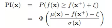
  思想：新的参数组合对应的目标函数值要高于历史的参数组合最优的

• 最大化提升期望(MEI, Maximize Expectation of Improvement)
  
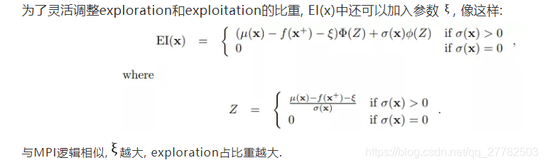
  思想：上述MPI的期望

2、最大化上置信界(Upper Confidence Bound)

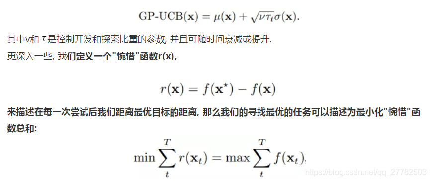
思想：将每次更新的参数对应的目标函数值和历史的目标函数值相减，定义为惋惜函数，最后再求和！最小化这个结果即可得到最优参数！

1.2 和前两种调参方式的区别

• 贝叶斯优化在每一步取样优化时都依据之前所有数据信息推断当前最佳尝试参数组合！
• 而不论是网格搜索还是随机搜索都没有利用之前的数据信息，每次调参之间是相互独立的！

2 贝叶斯调参原理

见上！

3 Python实现

主要使用到的库是 hyperopt ！

3.1 数据准备

为了方便大家复现, 我们使用kaggle比赛中的公共数据 “caravan-insurance-challenge.csv”. 该比赛旨在预测并解释客户购买房车旅行保险的可能性, 是一个典型的二元分类有监督学习.

每条记录并不是以"人"为单位而是以邮递地址为单位的"家庭"数据.
解释性特征有85个, 包括人口统计以及保险产品统计等方面的数据, 详情请参考以上数据链接

import pandas as pd # 数据处理
import numpy as np # 数据处理
import random #生成随机数
import lightgbm as lgb #lgbm模型
from sklearn.model_selection import KFold #n折交叉检验
import csv #用于结果输出与csv
from hyperopt import STATUS_OK # "status"

# 画图
import matplotlib.pyplot as plt
import seaborn as sns
%matplotlib inline

np.random.seed(123) #复现随机数
MAX_EVALS = 200 #调参过程迭代次数
N_FOLDS = 10 #10折交叉检验

# 读入数据
data = pd.read_csv('caravan-insurance-challenge.csv')
train = data[data['ORIGIN'] == 'train']
test = data[data['ORIGIN'] == 'test']

# 提取标签
train_labels = np.array(train['CARAVAN'].astype(np.int32)).reshape((-1,))
test_labels = np.array(test['CARAVAN'].astype(np.int32)).reshape((-1,))

# 删除多余字段
train = train.drop(columns = ['ORIGIN', 'CARAVAN'])
test = test.drop(columns = ['ORIGIN', 'CARAVAN'])

features = np.array(train)
test_features = np.array(test)
labels = train_labels[:]

print('Train shape: ', train.shape)
print('Test shape: ', test.shape)
train.head()

Train shape:  (5822, 85)
Test shape:  (4000, 85)

	MOSTYPE	MAANTHUI	MGEMOMV	MGEMLEEF	MOSHOOFD	MGODRK	MGODPR	MGODOV	MGODGE	MRELGE	...	ALEVEN	APERSONG	AGEZONG	AWAOREG	ABRAND	AZEILPL	APLEZIER	AFIETS	AINBOED	ABYSTAND
0	33	1	3	2	8	0	5	1	3	7	...	0	0	0	0	1	0	0	0	0	0
1	37	1	2	2	8	1	4	1	4	6	...	0	0	0	0	1	0	0	0	0	0
2	37	1	2	2	8	0	4	2	4	3	...	0	0	0	0	1	0	0	0	0	0
3	9	1	3	3	3	2	3	2	4	5	...	0	0	0	0	1	0	0	0	0	0
4	40	1	4	2	10	1	4	1	4	7	...	0	0	0	0	1	0	0	0	0	0

5 rows × 85 columns

data.groupby(['ORIGIN'])['CARAVAN'].mean()*100

ORIGIN
test     5.950000
train    5.977327
Name: CARAVAN, dtype: float64

检查标签占比情况, 我们发现购买保险的记录在训练集和测试集中仅约6%, 极度不平衡.
由于本文关注于调参, 将不纠结于处理不平衡数据的方法和特征工程(相关方法请期待后期分享), 只是选用AUC而非error rate作为衡量模型优劣的指标.

3.2 建模调参

3.2.1 基准线模型

疑问：roc_auc_score中两个参数是什么？一个是真实值没问题 一个是预测的 那究竟是预测的概率还是预测的值？

from sklearn.metrics import roc_auc_score
from timeit import default_timer as timer

# Model with default hyperparameters
model = lgb.LGBMClassifier()


start = timer()
model.fit(features, labels)
train_time = timer() - start

predictions = model.predict_proba(test_features)[:, 1]
auc = roc_auc_score(test_labels, predictions)

print(model)
print('\nThe baseline score on the test set is {:.4f}.'.format(auc))
print('The baseline training time is {:.4f} seconds'.format(train_time))

LGBMClassifier(boosting_type='gbdt', class_weight=None, colsample_bytree=1.0,
        importance_type='split', learning_rate=0.1, max_depth=-1,
        min_child_samples=20, min_child_weight=0.001, min_split_gain=0.0,
        n_estimators=100, n_jobs=-1, num_leaves=31, objective=None,
        random_state=None, reg_alpha=0.0, reg_lambda=0.0, silent=True,
        subsample=1.0, subsample_for_bin=200000, subsample_freq=0)

The baseline score on the test set is 0.7092.
The baseline training time is 0.3808 seconds

我们使用LGBM的默认超参数得到了测试集底线AUC≈0.7092

3.2.2 Hyperopt 调参

调参时, 我们需要准备好以下4个部分:

• 目标函数, 也就是我们的 $f(\boldsymbol{x})$, 这里是训练集的10折交叉检验的平均AUC. 由于Hyperopt进行的是最小值优化, 故考虑使用 1- AUC;
• 定义超参数空间;
• 优化算法: 先验假设(TPE)和采集函数(MEI);
• 调参过程记录.

3.2.3 目标函数

我们先来定义目标函数 $f(\boldsymbol{x})$, "objective".

• 入参: 参数组合"params";
• 出参: Hyperopt 中要求目标函数返回需要最小化的值"loss", 也就是交叉检验的平均(1-AUC); 以及"status" 指示过程是否成功.

由于训练集样本数据量少(<6000)我们可以放心使用10折交叉检验, 并为LGBM设置一个early_stopping为100, 使模型在连续100次没有进步的时候来强制结束训练.
为了使用 lgb.cv, 我们还需要创建lgb专用数据集, 如下:

#  lgb 数据集
train_set = lgb.Dataset(features, label = labels)

# 以下定义目标函数
def objective(params, n_folds = N_FOLDS):
    """Hyperopt 中 LGBM 的目标函数"""
    
    # 记录迭代次数
    global ITERATION    
    ITERATION += 1
    
    # 'boosting_type' 与 'subsample' 以来参数, 需要"unpack". 继续看'2.2.2'部分就明白了
    subsample = params['boosting_type'].get('subsample', 1.0)    
    params['boosting_type'] = params['boosting_type']['boosting_type']
    params['subsample'] = subsample
    
    # 确保超参数数值类型的正确性, 否侧Hyperopt会报错
    for parameter_name in ['num_leaves', 'subsample_for_bin', 'min_child_samples']:
        params[parameter_name] = int(params[parameter_name])
    
    start = timer()     
    # 进行10折交叉检验, 由于设置了early_stopping, num_boost_round设置相对高一些也不必担心
    cv_results = lgb.cv(params, train_set, num_boost_round = 10000, nfold = n_folds, 
                        early_stopping_rounds = 100, metrics = 'auc', seed = 50)    
    run_time = timer() - start
    
    # 找出cv中最大平均AUC
    best_score = np.max(cv_results['auc-mean'])
    loss = 1 - best_score
    
    # 最大平均AUC 对应的提升树的迭代次数
    n_estimators = int(np.argmax(cv_results['auc-mean']) + 1)

    # 将我们关心的结果输出至 csv 文件, 注意要用 'a', append
    of_connection = open(out_file, 'a')
    writer = csv.writer(of_connection)
    writer.writerow([loss, params, ITERATION, n_estimators, run_time])
    
    # 同时也可将结果存在返回结果中
    return {'loss': loss, 'params': params, 'iteration': ITERATION,
            'estimators': n_estimators, 
            'train_time': run_time, 'status': STATUS_OK}

3.2.4 定义超参数空间

我们选择上文打印出的默认参数中一下比较重要的10个参数进行调参, 如下:

import hyperopt
from hyperopt import hp
from hyperopt.pyll.stochastic import sample

# 定义超参数空间
space = {
    'class_weight': hp.choice('class_weight', [None, 'balanced']),
    'boosting_type': hp.choice('boosting_type', [{'boosting_type': 'gbdt', 'subsample': hp.uniform('gdbt_subsample', 0.5, 1)}, 
                                                 {'boosting_type': 'dart', 'subsample': hp.uniform('dart_subsample', 0.5, 1)},
                                                 {'boosting_type': 'goss', 'subsample': 1.0}]),
    'num_leaves': hp.quniform('num_leaves', 30, 150, 1),
    'learning_rate': hp.loguniform('learning_rate', np.log(0.01), np.log(0.2)),
    'subsample_for_bin': hp.quniform('subsample_for_bin', 20000, 300000, 20000),
    'min_child_samples': hp.quniform('min_child_samples', 20, 500, 5),
    'reg_alpha': hp.uniform('reg_alpha', 0.0, 1.0),
    'reg_lambda': hp.uniform('reg_lambda', 0.0, 1.0),
    'colsample_bytree': hp.uniform('colsample_by_tree', 0.6, 1.0)
}

Hyperopt 提供了10种定义参数空间的分布(详情可参考https://github.com/hyperopt/hyperopt/wiki/FMin):

• hp.choice(label, options): 离散的均匀分布, 适用于参数中类别的选择, 如"boosting_type"中选择"gbdt", "dart", "goss";
• hp.randint(label, upper): [0, upper) 定义域的整数均分布;
• hp.uniform(label, low, high): [low, high] 定义域的均匀分布;
• hp.quniform(label, low, high, q): round(uniform(low, high) / q) * q;
• hp.loguniform(label, low, high): exp(uniform(low, high)), 适用于夸量级的参数, 如learning_rate;
• hp.qloguniform(label, low, high, q): round(exp(uniform(low, high)) / q) * q;
• hp.normal(label, mu, sigma): 正态分布;
• hp.qnormal(label, mu, sigma, q): round(normal(mu, sigma) / q) * q;
• hp.lognormal(label, mu, sigma): exp(normal(mu, sigma));
• hp.qlognormal(label, mu, sigma, q): round(exp(normal(mu, sigma)) / q) * q;

3.2.5 优化算法

from hyperopt import tpe

# TPE + MEI 算法
tpe_algorithm = tpe.suggest

3.2.6 过程记录

在 2.2.2 目标函数的定义中, 我们同时用了两种记录方式, 分别可以用以下方式查看:

• 每次迭代写入csv中, 在迭代过程中可以使用 tail xxxx.csv来动态检查正在运行的优化代码;
• 以"return"方式返回的, 须使用Hyperopt的Trials实例在代码运行结束后查看, 具体操作如下.

from hyperopt import Trials
import os
# os.mkdir('results')

# csv 存储
out_file = 'results/gbm_trials.csv'
of_connection = open(out_file, 'w')
writer = csv.writer(of_connection)
writer.writerow(['loss', 'params', 'iteration', 'estimators', 'train_time']) # 制作表头 
of_connection.close()

# 利用 Trials 实例存储
bayes_trials = Trials()

• 知识点get制作excel表头！然后往里面写命令！
• import csv 然后csv.writer writer.writerow

3.2.7 优化结果

%%capture
from hyperopt import fmin

# 目标函数中的全局变量, 纪录迭代次数
global  ITERATION
ITERATION = 0

# 正式开始优化 
best = fmin(fn = objective, space = space, algo = tpe.suggest, 
            max_evals = MAX_EVALS, trials = bayes_trials, rstate = np.random.RandomState(50))

• objective是上面定义的目标函数
• space是用Hyperopt格式定义的需要调整的参数的组合
• algo为优化算法 即TPE+MEI 最大化提升期望
• max_evals 调参过程中迭代的最大次数 上面定义了 200
• trials：利用 Trials 实例存储
• rstate：设置随机数

bayes_results = pd.read_csv('results/gbm_trials.csv')
bayes_results.head()

	loss	params	iteration	estimators	train_time
0	0.244768	{'boosting_type': 'goss', 'class_weight': 'bal...	1	53	2.473031
1	0.274673	{'boosting_type': 'gbdt', 'class_weight': 'bal...	2	46	5.322019
2	0.241946	{'boosting_type': 'goss', 'class_weight': 'bal...	3	12	2.319422
3	0.239033	{'boosting_type': 'goss', 'class_weight': 'bal...	4	6	1.764528
4	0.231253	{'boosting_type': 'gbdt', 'class_weight': None...	5	182	6.053847

# bayes_results = pd.DataFrame(bayes_trials.results, columns=['loss', 'params', 'iteration', 'estimators', 'train_time'])
bayes_results.sort_values('loss', ascending = True, inplace = True)
bayes_results.reset_index(inplace = True, drop = True)
bayes_results.head()

	loss	params	iteration	estimators	train_time
0	0.230253	{'boosting_type': 'dart', 'class_weight': None...	67	781	1030.424565
1	0.230668	{'boosting_type': 'dart', 'class_weight': None...	70	657	951.559526
2	0.230767	{'boosting_type': 'gbdt', 'class_weight': None...	27	113	2.760706
3	0.231253	{'boosting_type': 'gbdt', 'class_weight': None...	5	182	6.053847
4	0.231589	{'boosting_type': 'dart', 'class_weight': None...	75	1313	964.707449

bayes_results.loc[0,'params']

"{'boosting_type': 'dart', 'class_weight': None, 'colsample_bytree': 0.6030976691881168, 'learning_rate': 0.015500349675709105, 'min_child_samples': 280, 'num_leaves': 35, 'reg_alpha': 0.27179070867537247, 'reg_lambda': 0.9098647782461072, 'subsample_for_bin': 160000, 'subsample': 0.8399482760565069}"

10折交叉检验中, 使用以上超参数最优平均loss达到了约0.230253. 现在我们来看一下这组最优参数在测试集的表现

best_bayes_params

"{'boosting_type': 'dart', 'class_weight': None, 'colsample_bytree': 0.6030976691881168, 'learning_rate': 0.015500349675709105, 'min_child_samples': 280, 'num_leaves': 35, 'reg_alpha': 0.27179070867537247, 'reg_lambda': 0.9098647782461072, 'subsample_for_bin': 160000, 'subsample': 0.8399482760565069}"

eval(best_bayes_params)

{'boosting_type': 'dart',
 'class_weight': None,
 'colsample_bytree': 0.6030976691881168,
 'learning_rate': 0.015500349675709105,
 'min_child_samples': 280,
 'num_leaves': 35,
 'reg_alpha': 0.27179070867537247,
 'reg_lambda': 0.9098647782461072,
 'subsample_for_bin': 160000,
 'subsample': 0.8399482760565069}

# 取最优参数
import copy
best_bayes_estimators = int(bayes_results.loc[0, 'estimators'])
best_bayes_params = bayes_results.loc[0, 'params']

# 使用全量训练集建模
best_bayes_model = lgb.LGBMClassifier(n_estimators=best_bayes_estimators, n_jobs = -1, 
                                       objective = 'binary', random_state = 50, **eval(best_bayes_params))
best_bayes_model.fit(features, labels)

# 测试机表现
preds = best_bayes_model.predict_proba(test_features)[:, 1]
print('Bayes优化测试集AUC: {:.5f}.'.format(roc_auc_score(test_labels, preds)))
print('使用 {} 树达到该效果'.format(bayes_results.loc[0, 'estimators']))

Bayes优化测试集AUC: 0.72548.
使用 781 树达到该效果

注，由于迭代次数太多，中途停止了，上述应该不是最优！但思路和代码都没有问题！

bayes_results['train_time'].sum()/60

1391.6635087600323

200次贝叶斯优化迭代共耗时约1392分钟, 找到的参数组合使用781棵树达到AUC≈0.7255的结果, 对比基线模型100棵树的0.7092确实有所提高.

4 参考

• https://mp.weixin.qq.com/s/wHtiZlzHENCcLXosOA3Xbw
• http://blog.sina.com.cn/s/blog_a7c687210102wv41.html
• http://blog.sina.com.cn/s/blog_a7c687210102wv3t.html