本篇是基于jdk8(要想技术深,源码必须看),
网上对hashmap的介绍很多,借鉴之前的大神们的杰作并基于自己的理解总结,由于时间紧凑,简洁精炼。
源码中开始注释的一大段(翻译出来):
/*
 * Implementation notes.
 *
 * This map usually acts as a binned (bucketed) hash table, but
 * when bins get too large, they are transformed into bins of
 * TreeNodes, each structured similarly to those in
 * java.util.TreeMap. Most methods try to use normal bins, but
 * relay to TreeNode methods when applicable (simply by checking
 * instanceof a node).  Bins of TreeNodes may be traversed and
 * used like any others, but additionally support faster lookup
 * when overpopulated. However, since the vast majority of bins in
 * normal use are not overpopulated, checking for existence of
 * tree bins may be delayed in the course of table methods.
 *
 * Tree bins (i.e., bins whose elements are all TreeNodes) are
 * ordered primarily by hashCode, but in the case of ties, if two
 * elements are of the same "class C implements Comparable<C>",
 * type then their compareTo method is used for ordering. (We
 * conservatively check generic types via reflection to validate
 * this -- see method comparableClassFor).  The added complexity
 * of tree bins is worthwhile in providing worst-case O(log n)
 * operations when keys either have distinct hashes or are
 * orderable, Thus, performance degrades gracefully under
 * accidental or malicious usages in which hashCode() methods
 * return values that are poorly distributed, as well as those in
 * which many keys share a hashCode, so long as they are also
 * Comparable. (If neither of these apply, we may waste about a
 * factor of two in time and space compared to taking no
 * precautions. But the only known cases stem from poor user
 * programming practices that are already so slow that this makes
 * little difference.)
 *
 * Because TreeNodes are about twice the size of regular nodes, we
 * use them only when bins contain enough nodes to warrant use
 * (see TREEIFY_THRESHOLD). And when they become too small (due to
 * removal or resizing) they are converted back to plain bins.  In
 * usages with well-distributed user hashCodes, tree bins are
 * rarely used.  Ideally, under random hashCodes, the frequency of
 * nodes in bins follows a Poisson distribution
 * (http://en.wikipedia.org/wiki/Poisson_distribution) with a
 * parameter of about 0.5 on average for the default resizing
 * threshold of 0.75, although with a large variance because of
 * resizing granularity. Ignoring variance, the expected
 * occurrences of list size k are (exp(-0.5) * pow(0.5, k) /
 * factorial(k)). The first values are:
 *
 * 0:    0.60653066
 * 1:    0.30326533
 * 2:    0.07581633
 * 3:    0.01263606
 * 4:    0.00157952
 * 5:    0.00015795
 * 6:    0.00001316
 * 7:    0.00000094
 * 8:    0.00000006
 * more: less than 1 in ten million
 *
 * The root of a tree bin is normally its first node.  However,
 * sometimes (currently only upon Iterator.remove), the root might
 * be elsewhere, but can be recovered following parent links
 * (method TreeNode.root()).
 *
 * All applicable internal methods accept a hash code as an
 * argument (as normally supplied from a public method), allowing
 * them to call each other without recomputing user hashCodes.
 * Most internal methods also accept a "tab" argument, that is
 * normally the current table, but may be a new or old one when
 * resizing or converting.
 *
 * When bin lists are treeified, split, or untreeified, we keep
 * them in the same relative access/traversal order (i.e., field
 * Node.next) to better preserve locality, and to slightly
 * simplify handling of splits and traversals that invoke
 * iterator.remove. When using comparators on insertion, to keep a
 * total ordering (or as close as is required here) across
 * rebalancings, we compare classes and identityHashCodes as
 * tie-breakers.
 *
 * The use and transitions among plain vs tree modes is
 * complicated by the existence of subclass LinkedHashMap. See
 * below for hook methods defined to be invoked upon insertion,
 * removal and access that allow LinkedHashMap internals to
 * otherwise remain independent of these mechanics. (This also
 * requires that a map instance be passed to some utility methods
 * that may create new nodes.)
 *
 * The concurrent-programming-like SSA-based coding style helps
 * avoid aliasing errors amid all of the twisty pointer operations.
 */
实现注意事项。
这个映射通常充当一个binned (bucked)哈希表,但是
当箱子变得太大时,它们就变成了
树状结构,每一种结构都类似于
java.util.TreeMap。大多数方法都尝试使用普通的箱子,但是
在适用时转发到TreeNode方法(只需检查即可)
实例一个节点)。可以遍历和
与其他任何方法一样使用,但还支持更快的查找
当人口过剩。不过,由于绝大多数垃圾桶都在
正常使用时不超载,检查是否存在
在表方法的过程中,可能会延迟树容器。
树垃圾箱(即。,其元素都为树节点的桶)
主要按hashCode排序,但如果是tie,则是两个
元素是相同的“类C实现可比的<C>”,
然后使用它们的compareTo方法进行排序。(我们
通过反射保守地检查泛型类型以验证
这个——参见方法comparableClassFor)。增加了复杂性
提供最坏情况O(log n)是值得的
当键具有不同的哈希值或为
因此,可排序的性能会优雅地下降
hashCode()方法的意外或恶意使用
返回分布不好的值,以及in中的值
哪些键共享一个hashCode,只要它们也是
具有可比性。如果这两种方法都不适用,我们可能会浪费a
因子2在时间和空间上比取no
预防措施。但目前所知的情况只有可怜的用户
编程实践已经非常缓慢,这使得
小的区别。)
因为树节点的大小大约是普通节点的两倍,所以我们
只有当容器中包含足够的节点以保证使用时才使用它们
(见TREEIFY_THRESHOLD)。当它们变得太小的时候
移除或调整大小)它们被转换回普通的箱子。在
使用分布良好的用户哈希码,树箱是
很少使用。理想情况下,在随机哈希码下
箱中的节点遵循泊松分布
(http://en.wikipedia.org/wiki/Poisson_distribution)
默认大小调整的参数平均约为0.5
阈值为0.75,虽然由于方差较大
调整粒度。忽略方差,得到期望
列表大小k的出现次数为(exp(-0.5) * pow(0.5, k) /
阶乘(k))。第一个值是:
0:0.60653066
1:0.30326533
2:0.07581633
3:0.01263606
4:0.00157952
5:0.00015795
6:0.00001316
7:0.00000094
8:0.00000006
多于:少于千分之一
树状容器的根通常是它的第一个节点。然而,
有时(当前仅在Iterator.remove上),根可能
在其他位置,但可以通过父链接恢复
(方法TreeNode.root ())。
所有适用的内部方法都接受哈希码作为
参数(通常由公共方法提供),允许
它们可以在不重新计算用户哈希码的情况下相互调用。
也就是说,大多数内部方法也接受“tab”参数
通常是当前表,但可能是新表或旧表时
调整或转换。
当bin列表被treeified、split或untreeified时,我们保存
它们的相对访问/遍历顺序相同(即、现场
为了更好地保存局部,稍微
简化对调用的拆分和遍历的处理
iterator.remove。当使用比较器插入时,要保持a
跨区域的总排序(或与此处所需的最接近)
重新平衡时,我们将类和标识哈希码进行比较
参加。
在普通模式和树模式之间的使用和转换是
由于LinkedHashMap子类的存在而变得复杂。看到
下面是定义在插入时调用的钩子方法,
删除和访问允许LinkedHashMap内部文件
否则将独立于这些机制之外。(这也
要求将映射实例传递给一些实用程序方法
这可能会创建新的节点。)
基于并行编程的类似于ssa的编码风格很有帮助
避免所有扭曲指针操作中的混叠错误。
1、 hashmap特点:很多都爱和hashtable进行对比,如果面试问道和hashtable比较,那太简单了,hashmap是一种基于hash算法存储key-value的键值对。可以存储null,注意是键和值都可以为null。(疑问1:为null的键放在哪了?),线程非安全。
2、存储结构:数组和链表的结合体,
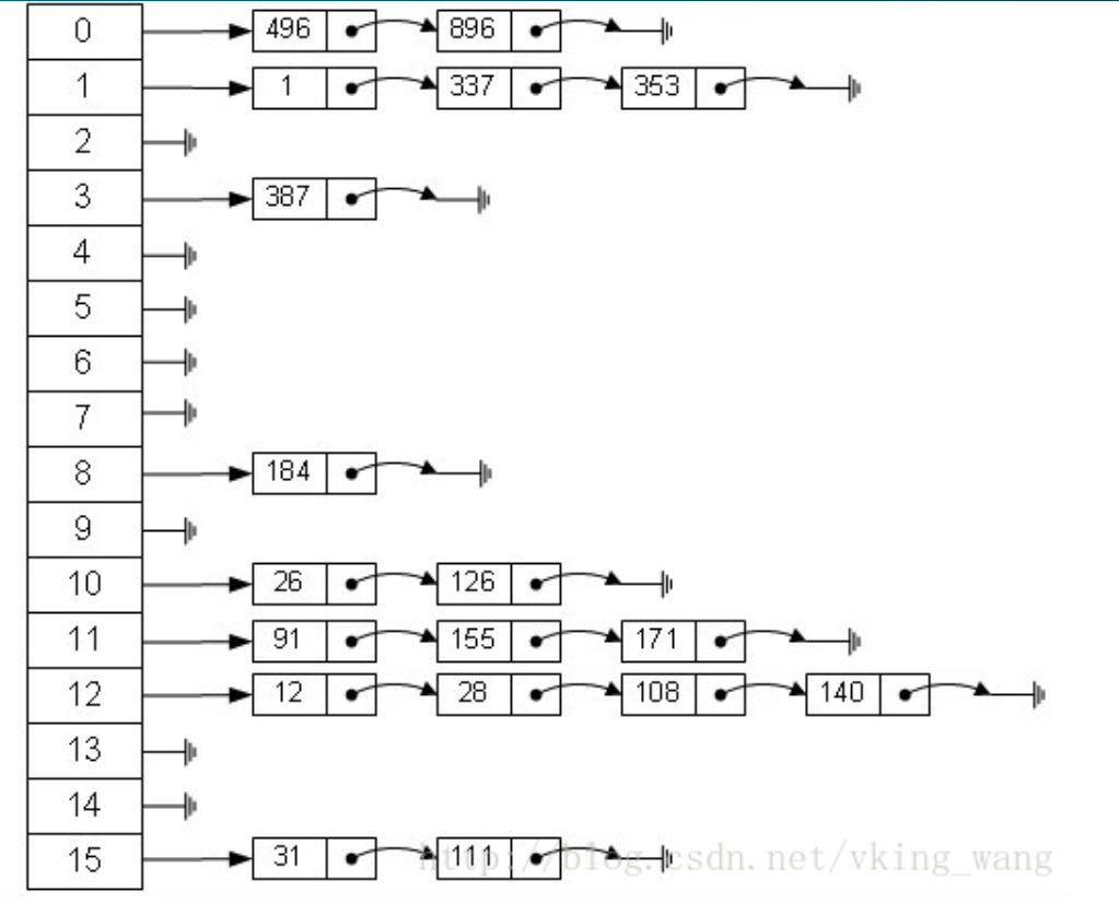
 3、 从图中(借用别人的图)可以看出,0-15是数组,后面的是链表,数组时Map.Entry<K,V>,链表是Node<K,V>,两个结构后续讲解。hashmap继承AbstractMap,实现map接口、cloneable接口、Serializable接口,只要是可以对已有的map进行clone操作和序列化和反序列化操作。
属性:
3.1 static final int DEFAULT_INITIAL_CAPACITY = 1 << 4:hashmap的默认初始化容量16,这里用位移运算符,增快效率
3.2 static final int MAXIMUM_CAPACITY = 1 << 30:hashmap的最大容量,为int的最大值。同样适用位移运算符
3.3 static final float DEFAULT_LOAD_FACTOR = 0.75f:扩容因子,决定扩容的因素之一,一种折中的取值
3.4 static final int TREEIFY_THRESHOLD = 8:链表节点超过8个是进行红黑树的转换
3.5 static final int UNTREEIFY_THRESHOLD = 6:由树转换成链表的阈值
3.6
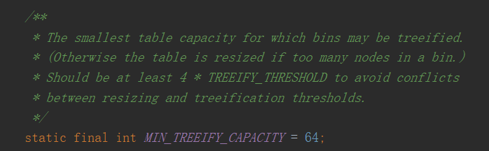
当哈希表中的容量大于这个值时,表中的桶才能进行树形化 ,否则桶内元素太多时会扩容,而不是树形化,为了避免进行扩容、树形化选择的冲突,这个值不能小于 4 * TREEIFY_THRESHOLD,换句话说,不是每个数组上的链表节点数量大于8就一定树形化
4、构造方法:
4.1
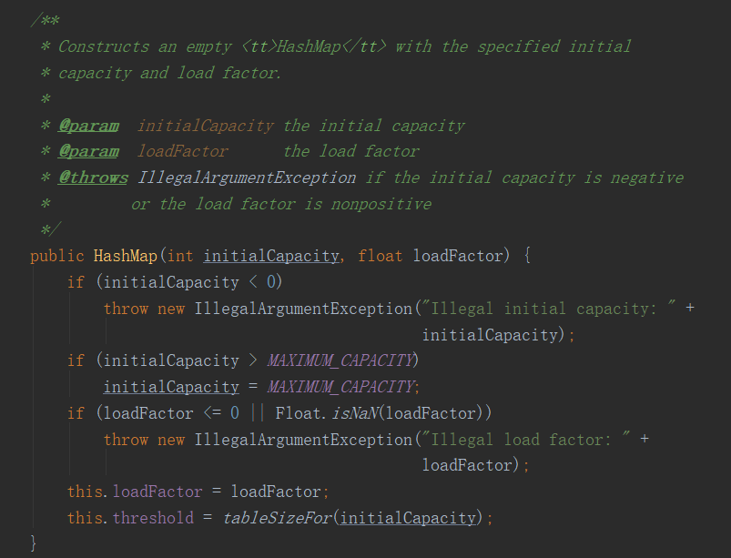
此构造方法传入两个方法,第一个是初始容量,第二个是扩容因子。首先,判断初始容量是否小于0,小于0则抛出异常,如果大于MAXIMUM_CAPACITY ,则赋予其MAXIMUM_CAPACITY 。
如果扩容因子小于等于0且是不确定性数据时(NaN,Not a Number),抛出异常。都不是则进行赋值操作。
4.2

此构造方法中只传一个初始容量,扩容因子取默认,并调用4.1中的构造方法
4.3

此构造方法时不传任何方法的数据,构造一个默认容量为16,扩容因子为0.75f的hashmap
4.4
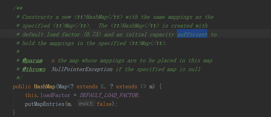
此构造方法中创建了一个将特定的map中数据放到新创建的map中。
5、hashmap重要方法详解
5.1 put 方法

此方法中调用了另一个构造方法,

(重点来了,面试的重点):首先创建Node<K,V>[] tab; Node<K,V> p; int n, i这些值,如果table的为null或者大小为0,则没有创建hashmap,通过resize方法进行初始化大小,由于hashmap为null,所以table也为null,则进行第一次的调整大小为默认容量为16,扩容因子为0.75f。具体流程可以参考下面的流程图:

有一个重点是key为null的key放在哪了,放在了下表为0的位置上。
5.2 get方法

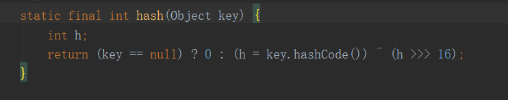
hash方法有一个注释翻译过来:
计算key.hashCode()并传播(XORs)更高的散列位
降低。因为表使用的是2的幂掩码,所以是
仅在当前掩码之上的位上变化的散列将会
总是发生碰撞。(已知的例子中有一组浮点键
在小表格中保存连续的整数。)所以我们
应用一个转换来扩展更高位的影响
向下。在速度、效用和之间有一个权衡
bit-spreading质量。因为有很多常见的哈希值
已经被合理地分配了(所以没有从中受益
因为我们用树木来处理大量的树木
箱子里的碰撞,我们只是平移了一些位
最便宜的方法,以减少系统损失,以及
以吸收最高位的影响,否则会
由于表的边界,永远不要在索引计算中使用。
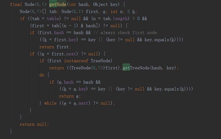
看方法分析:1、先判断table是否为空?为空则直接返回null,不为空直接入第二步
2、计算key的hash值,key的hash值是将key的hashcode与齐值的无符号右移16位的或结果,起作用能获得更好的散列值,然后通过计算后的hash值与table的长度-1进行与计算,得到key对应的value可能存在的链表Entry的入口位置,即头结点
3、对头结点判断hash值是否相等且通过equals方法判断key相等否?相等直接返回,不相等则进入第四步
4、头结点不等于空,判断是否为红黑树节点,如果是红黑树,则通过遍历红黑树进行寻找值,如果不是红黑树,则进行第五步
5、遍历链表节点进行查找key值,找到返回,没找到返回null