[C2]逻辑回归

逻辑回归（Logistic Regression）

假设函数（Hypothesis Function）

$h_\theta(x)=g(\theta^Tx)=g(z)=\frac{1}{1+e^{-z}}=\frac{1}{1+e^{\theta^Tx}}$

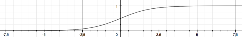
g函数称为 Sigmoid Function 或 Logistic Function, 它可以使得 $0 \leq h_\theta (x) \leq 1$.

The following image shows us what the sigmoid function looks like:

$h_\theta(x)$ 用来估计基于输入特征值x，y=1的可能性。正式的写法为：

$h_\theta(x)=P(y=1|x;\theta)=1-P(y=0|x;\theta)$

因为
$z=0,e^0=1 \implies g(z) = \frac{1}{2}$
$z \to \infty,e^{-\infty} \to 0 \implies g(z) = 1$
$z \to - \infty,e^{\infty} \to \infty \implies g(z) = 0$

所以
当 $h_\theta(x) \geq 0.5$ 或 $z \geq 0$ 时，y=1
当 $h_\theta(x) < 0.5$ 或 $z < 0$ 时，y=0

另外
The input to the sigmoid function g(z) (e.g. $\theta^T X$) doesn't need to be linear, and could be a function that describes a circle (e.g. $z = \theta_0 + \theta_1 x_1^2 +\theta_2 x_2^2$) or any shape to fit our data.

代价函数（Cost Function）

We cannot use the same cost function that we use for linear regression because the Logistic Function will cause the output to be wavy, causing many local optima. In other words, it will not be a convex function.

Instead, our cost function for logistic regression looks like:

$J(\theta)=\frac{1}{m} \sum\limits_{i=1}^m Cost(h_\theta(x^{(i)}),y^{(i)})$

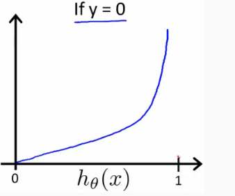
$\begin{cases} Cost(h_\theta(x),y)=-log(h_\theta(x)) & \quad \text{if y = 1} \\ \\ Cost(h_\theta(x),y)=-log(1-h_\theta(x)) & \quad \text{if y = 0} \end{cases}$

When y = 1, we get the following plot for $J(\theta)$ vs $h_\theta (x)$:

Similarly, when y = 0, we get the following plot for J(θ) vs hθ(x):

If our correct answer 'y' is 1, then the cost function will be 0 if our hypothesis function outputs 1. If our hypothesis approaches 0, then the cost function will approach infinity.
当 $y=1$ 时，若 $h_\theta(x)=1$ ，则 $Cost=0$ ，若 $h_\theta(x)=0$ ，则 $Cost \to \infty$；

If our correct answer 'y' is 0, then the cost function will be 0 if our hypothesis function also outputs 0. If our hypothesis approaches 1, then the cost function will approach infinity.
当 $y=0$ 时，若 $h_\theta(x)=0$ ，则 $Cost=0$ ，若 $h_\theta(x)=1$ ，则 $Cost \to \infty$。

Note that writing the cost function in this way guarantees that J(θ) is convex for logistic regression.
这种代价函数的表示方法可以确保逻辑回归的 $J(\theta)$ 是凸函数，所以可以使用梯度下降求解 $\theta$

将 $Cost \Big(h_\theta(x),y \Big)$ 简化可得（We can compress our cost function's two conditional cases into one case）：

$Cost \Big(h_\theta(x),y \Big)=-y \cdot log \Big(h_\theta(x) \Big) - (1-y) \cdot log \Big(1-h_\theta(x) \Big)$

最终的代价函数为（We can fully write out our entire cost function as follows）：

$J(\theta)=-\frac{1}{m} \sum\limits_{i=1}^m \Bigg[ y^{(i)} \cdot log \bigg(h_\theta(x^{(i)}) \bigg) + (1-y^{(i)}) \cdot log \bigg(1-h_\theta(x^{(i)}) \bigg) \Bigg]$

向量化表示为（A vectorized implementation is）：

$\overrightarrow{h}=g(X \overrightarrow{\theta})$

$J(\theta)=\frac{1}{m} \cdot \Big( -\overrightarrow{y}^T \cdot log(\overrightarrow{h}) - (1- \overrightarrow{y})^T \cdot log(1- \overrightarrow{h}) \Big)$

梯度下降（Gradient Descent）

重复，直到收敛（Repeat until convergence）：

$\theta_j := \theta_j - \alpha\frac{\partial}{\partial\theta_j}J(\theta_0,\theta_1,···\theta_n)$, 其中 $\frac{\partial}{\partial\theta_j}J(\theta_0,\theta_1,···\theta_n)$ 计算方法为对 $\theta_j$ 求偏导数（partial derivative）

即（We can work out the derivative part using calculus to get）：

$\theta_j := \theta_j - \alpha\frac{1}{m}\sum\limits_{i = 1}^{m}\biggl(h_\theta(x^{(i)}) - y^{(i)}\biggl)\cdot x_j^{(i)}$

同时更新（simultaneously update）$\theta_j$, for j = 0, 1 ..., n

另外， $x_0^{(i)} \equiv 1$

向量化表示为（A vectorized implementation is）：

$\theta := \theta - \frac{\alpha}{m} X^T \Big( g(X\theta) - \overrightarrow{y} \Big)$

Advanced Optimization for Gradient Descent

除了梯度下降法外，还有其他方法计算 $\overrightarrow{\theta}$ ：

共轭梯度法（Conjugate gradient）
变长度法（BFGS）
限制尺度法（L-BFGS）

优点是，无需手动选择学习速率 $\alpha$ , 以及收敛速度更快。缺点是更加的复杂。

Octave 中已经有提供该方法（fminunc），要调用 fminunc 方法来计算 $\overrightarrow{\theta}$，需先计算 $J(\theta)$ 和 $\frac{\alpha}{\alpha \theta_j}J(\theta)$

可以写一个简单的函数返回这两个值

function [jVal, gradient] = costFunction(theta)
  jVal = [...code to compute J(theta)...];
  gradient = [...code to compute derivative of J(theta)...];
end

然后使用Octave的“fminunc()”优化算法以及“optimset()”函数来创建一个包含要发送到“fminunc()”的“options“对象。

options = optimset('GradObj', 'on', 'MaxIter', 100);
initialTheta = zeros(2,1); % our initial vector of theta values
[optTheta, functionVal, exitFlag] = fminunc(@costFunction, initialTheta, options);

多元分类（Multiclass Classification: One-vs-all）

对于多元分类的情况，即 y = {0,1...n}，我们可以把问题分解为 n+1 个二元分类的问题。 +1 是因为索引是从0开始的。

$y \in $ {0,1...n}

$h_\theta^{(0)}(x)=P(y=0|x;\theta)$

$h_\theta^{(1)}(x)=P(y=1|x;\theta)$

$...$

$h_\theta^{(n)}(x)=P(y=n|x;\theta)$

$prediction=\max\limits_i(h_\theta^{(i)}(x))$

我们基本上是选择一个类，然后把所有其他类都放到第二类中。重复这样做，对每种情况应用二元逻辑回归，然后使用返回最大值的假设作为我们的预测。

The following image shows how one could classify 3 classes:

To summarize:

Train a logistic regression classifier $h_\theta(x)$ for each class to predict the probability that y = i .

To make a prediction on a new x, pick the class that maximizes $h_\theta (x)$

程序代码

直接查看Logistic Regression.ipynb可点击

获取源码以其他文件，可点击右上角 Fork me on GitHub 自行 Clone。