收入囊中
- 拉普拉斯算子
- LOG算子(高斯拉普拉斯算子)
- OpenCV Laplacian函数
- 构建自己的拉普拉斯算子
- 利用拉普拉斯算子进行图像的锐化
葵花宝典
在OpenCV2马拉松第14圈——边缘检测(Sobel,prewitt,roberts)
我们已经认识了3个一阶差分算子
拉普拉斯算子是二阶差分算子,为什么要加入二阶的算子呢?试想一下,如果图像中有噪声,噪声在一阶导数处也会取得极大值从而被当作边缘。然而求解这个极大值也不方便,采用二阶导数后,极大值点就为0了,因此值为0的地方就是边界。
有图有真相!
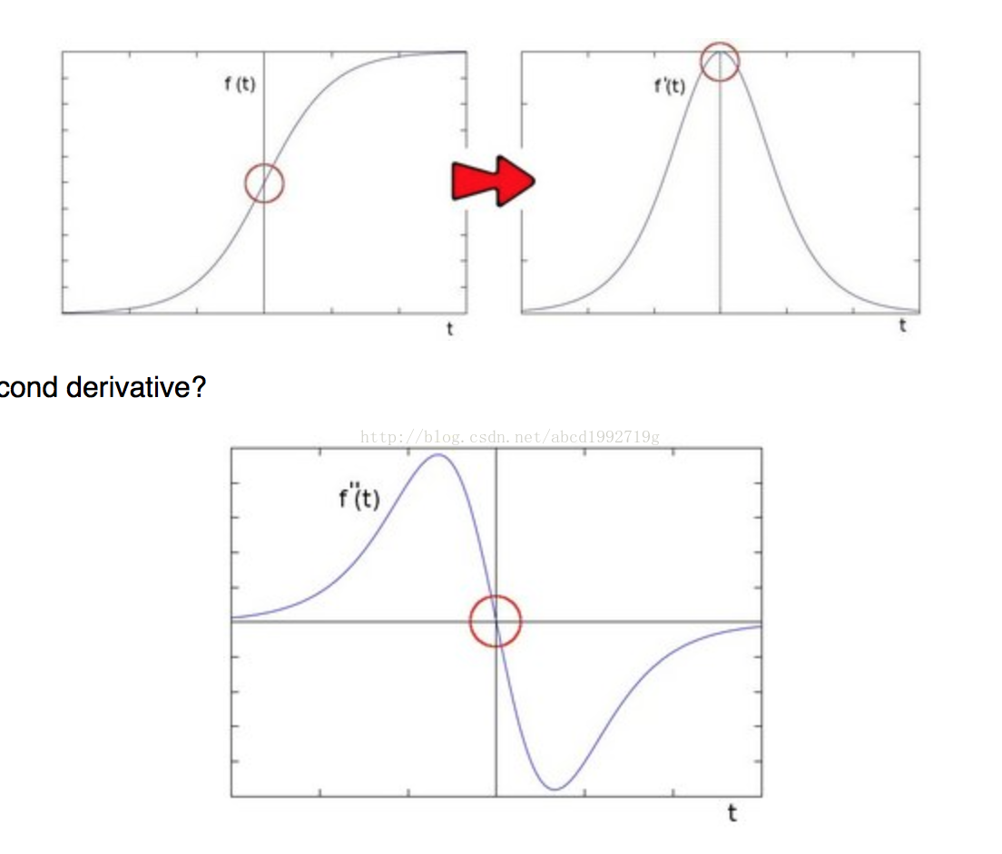 上面是一阶导数,下面是二阶导数
离散形式:
| |
 |
| 图5-9 拉普拉斯的4种模板 |
拉普拉斯算子会放大噪声,因此我们采用了LOG算子,就是高斯拉普拉斯算子,先对图像进行高斯模糊,抑制噪声,再求二阶导数,二阶导数为0的地方就是图像的边界。
初识API
API不用解释了,和Sobel完全一样!
- C++: void Laplacian (InputArray src, OutputArray dst, int ddepth, int ksize=1, double scale=1, double delta=0, int borderType=BORDER_DEFAULT )
-
- src – Source image.
- dst – Destination image of the same size and the same number of channels as src .
- ddepth – Desired depth of the destination image.
- ksize – Aperture size used to compute the second-derivative filters. See getDerivKernels() for details. The size must be positive and odd.
- scale – Optional scale factor for the computed Laplacian values. By default, no scaling is applied. See getDerivKernels() for details.
- delta – Optional delta value that is added to the results prior to storing them in dst .
- borderType – Pixel extrapolation method. See borderInterpolate() for details.
This is done when ksize > 1 . When ksize == 1 , the Laplacian is computed by filtering the image with the following  aperture:

荷枪实弹
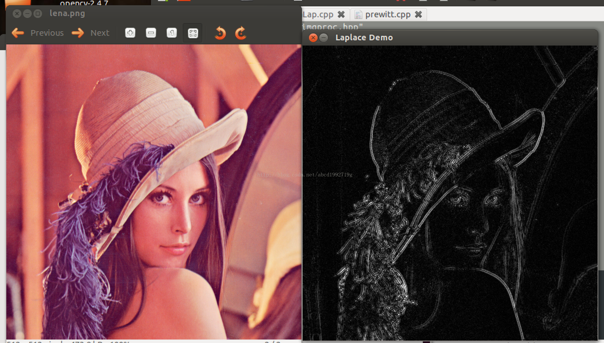
我们先调用API来实现
#include "opencv2/imgproc/imgproc.hpp"
#include "opencv2/highgui/highgui.hpp"

using namespace cv;

int main( int, char** argv )
{

  Mat src, src_gray;
  int kernel_size = 3;
  const char* window_name = "Laplace Demo";

  src = imread( argv[1] );
  GaussianBlur( src, src, Size(3,3), 0, 0, BORDER_DEFAULT );
  cvtColor( src, src_gray, CV_RGB2GRAY );
  namedWindow( window_name, CV_WINDOW_AUTOSIZE );

  Mat dst, abs_dst;
  Laplacian( src_gray, dst, CV_16S, kernel_size);
  convertScaleAbs( dst, abs_dst );

  imshow( window_name, abs_dst );
  waitKey(0);
  return 0;
}
效果图:
下面,我们用之前讲过的自定义滤波实现,采用
| 1 | 1 | 1 |
| 1 | -8 | 1 |
| 1 | 1 | 1 |
#include "opencv2/highgui/highgui.hpp"
#include "opencv2/imgproc/imgproc.hpp"
using namespace cv;

int main( int, char** argv )
{
	Mat src,gray,Kernel;

    src = imread( argv[1] );
    GaussianBlur( src, src, Size(3,3), 0, 0, BORDER_DEFAULT );
    cvtColor( src, gray, CV_RGB2GRAY );
    namedWindow("dstImage", 1);

    Kernel = (Mat_<double>(3,3) << 1, 1, 1, 1, -8, 1, 1, 1, 1);
    Mat grad,abs_grad;
    filter2D(gray, grad, CV_16S , Kernel, Point(-1,-1));
    convertScaleAbs( grad, abs_grad );

    imshow("dstImage", abs_grad);
    waitKey();
    return 0;
}
效果图就不发了,跟上面差不多
举一反三
拉普拉斯算子有没有跟多的应用,当然有,比如图像锐化。
由于拉普拉斯是一种微分算子,它可增强图像中灰度突变的区域,减弱灰度的缓慢变化区域。因此,锐化处理可选择拉普拉斯算子对原图像进行处理,产生描述灰度突变的图像,再将拉普拉斯图像与原始图像叠加而产生锐化图像。拉普拉斯锐化的基本方法可以由下式表示:
 |
锐化代码
#include "opencv2/highgui/highgui.hpp"
#include "opencv2/imgproc/imgproc.hpp"
using namespace cv;

int main( int, char** argv )
{
    Mat src,gray;

    src = imread( argv[1] );
    GaussianBlur( src, src, Size(3,3), 0, 0, BORDER_DEFAULT );
    cvtColor( src, gray, CV_RGB2GRAY );
    namedWindow("srcImage", 1);
    namedWindow("dstImage", 1);

    Mat grad,abs_grad;
    Laplacian( gray, grad, CV_16S, 3);
    convertScaleAbs( grad, abs_grad );
    Mat sharpped = gray + abs_grad;

    imshow("srcImage", gray);
    imshow("dstImage", sharpped);
    waitKey();
    return 0;
}
效果图:
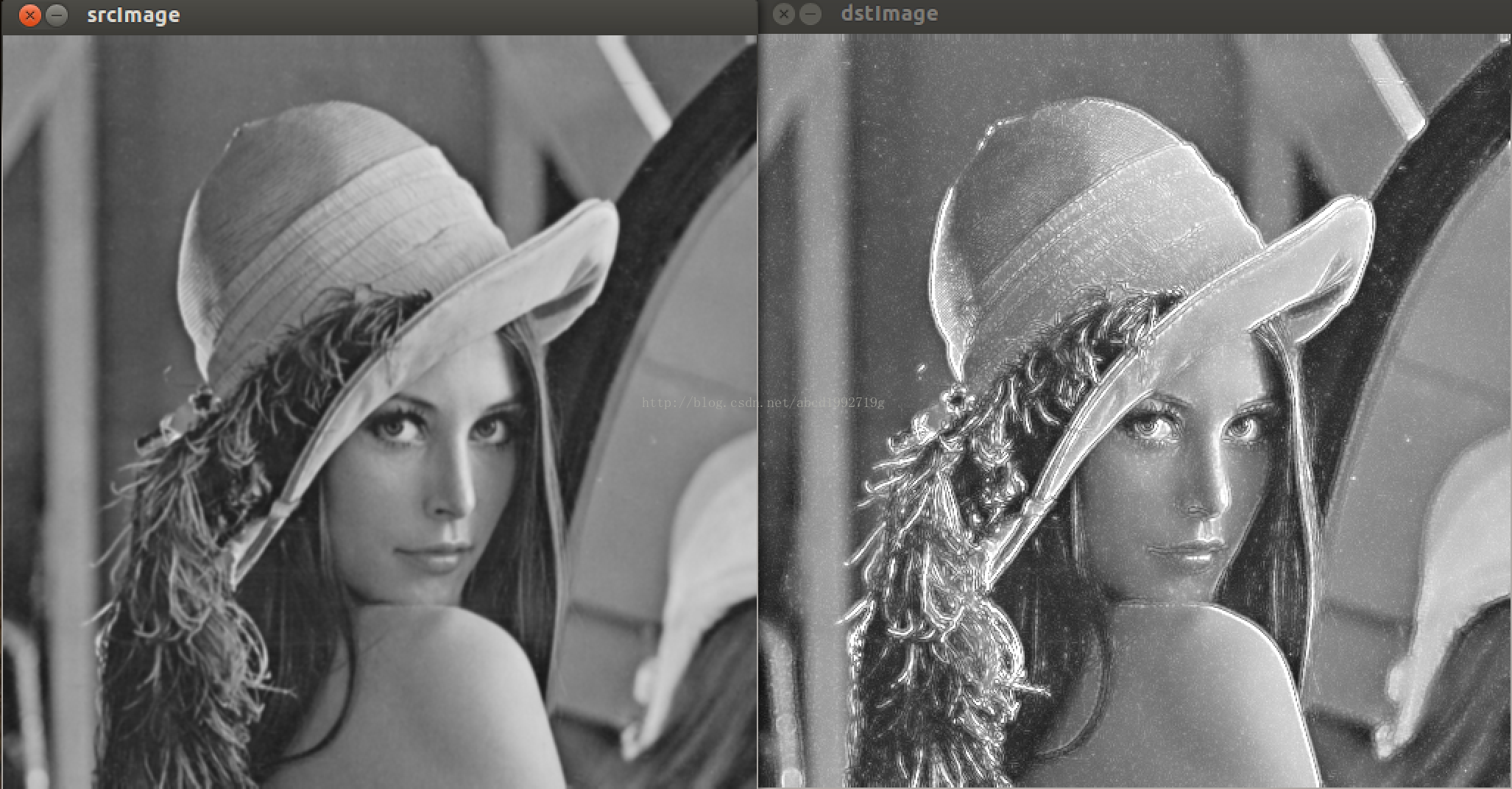
有放大噪声(很难避免)