Minimization of risk and maximization of profit on behalf of the bank.
To minimize loss from the bank’s perspective, the bank needs a decision rule regarding who to give approval of the loan and who not to. An applicant’s demographic and socio-economic profiles are considered by loan managers before a decision is taken regarding his/her loan application.
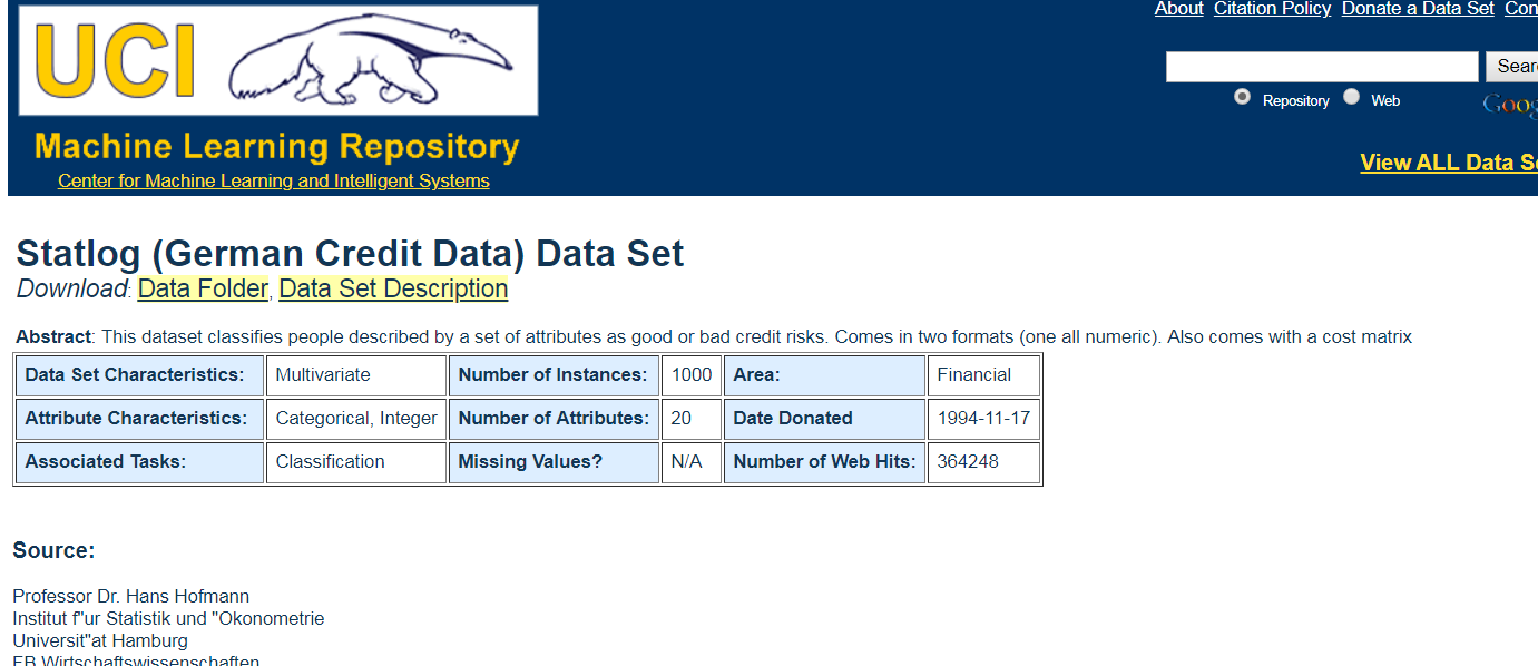
The German Credit Data contains data on 20 variables and the classification whether an applicant is considered a Good or a Bad credit risk for 1000 loan applicants. Here is a link to the German Credit data (right-click and "save as" ). A predictive model developed on this data is expected to provide a bank manager guidance for making a decision whether to approve a loan to a prospective applicant based on his/her profiles.
信用评分系统应用
http://archive.ics.uci.edu/ml/datasets/Statlog+(German+Credit+Data)
account balance 账户余额
duration of credit

Data Set Information:
Two datasets are provided. the original dataset, in the form provided by Prof. Hofmann, contains categorical/symbolic attributes and is in the file "german.data".
For algorithms that need numerical attributes, Strathclyde University produced the file "german.data-numeric". This file has been edited and several indicator variables added to make it suitable for algorithms which cannot cope with categorical variables. Several attributes that are ordered categorical (such as attribute 17) have been coded as integer. This was the form used by StatLog.
This dataset requires use of a cost matrix (see below)
..... 1 2
----------------------------
1 0 1
-----------------------
2 5 0
(1 = Good, 2 = Bad)
The rows represent the actual classification and the columns the predicted classification.
It is worse to class a customer as good when they are bad (5), than it is to class a customer as bad when they are good (1).
Attribute Information:
Attribute 1: (qualitative)
Status of existing checking account
A11 : ... < 0 DM
A12 : 0 <= ... < 200 DM
A13 : ... >= 200 DM / salary assignments for at least 1 year
A14 : no checking account
Attribute 2: (numerical)
Duration in month
Attribute 3: (qualitative)
Credit history
A30 : no credits taken/ all credits paid back duly
A31 : all credits at this bank paid back duly
A32 : existing credits paid back duly till now
A33 : delay in paying off in the past
A34 : critical account/ other credits existing (not at this bank)
Attribute 4: (qualitative)
Purpose
A40 : car (new)
A41 : car (used)
A42 : furniture/equipment
A43 : radio/television
A44 : domestic appliances
A45 : repairs
A46 : education
A47 : (vacation - does not exist?)
A48 : retraining
A49 : business
A410 : others
Attribute 5: (numerical)
Credit amount
Attibute 6: (qualitative)
Savings account/bonds
A61 : ... < 100 DM
A62 : 100 <= ... < 500 DM
A63 : 500 <= ... < 1000 DM
A64 : .. >= 1000 DM
A65 : unknown/ no savings account
Attribute 7: (qualitative)
Present employment since
A71 : unemployed
A72 : ... < 1 year
A73 : 1 <= ... < 4 years
A74 : 4 <= ... < 7 years
A75 : .. >= 7 years
Attribute 8: (numerical)
Installment rate in percentage of disposable income
Attribute 9: (qualitative)
Personal status and sex
A91 : male : divorced/separated
A92 : female : divorced/separated/married
A93 : male : single
A94 : male : married/widowed
A95 : female : single
Attribute 10: (qualitative)
Other debtors / guarantors
A101 : none
A102 : co-applicant
A103 : guarantor
Attribute 11: (numerical)
Present residence since
Attribute 12: (qualitative)
Property
A121 : real estate
A122 : if not A121 : building society savings agreement/ life insurance
A123 : if not A121/A122 : car or other, not in attribute 6
A124 : unknown / no property
Attribute 13: (numerical)
Age in years
Attribute 14: (qualitative)
Other installment plans
A141 : bank
A142 : stores
A143 : none
Attribute 15: (qualitative)
Housing
A151 : rent
A152 : own
A153 : for free
Attribute 16: (numerical)
Number of existing credits at this bank
Attribute 17: (qualitative)
Job
A171 : unemployed/ unskilled - non-resident
A172 : unskilled - resident
A173 : skilled employee / official
A174 : management/ self-employed/
highly qualified employee/ officer
Attribute 18: (numerical)
Number of people being liable to provide maintenance for
Attribute 19: (qualitative)
Telephone
A191 : none
A192 : yes, registered under the customers name
Attribute 20: (qualitative)
foreign worker
A201 : yes
A202 : no
It is worse to class a customer as good when they are bad (5),
than it is to class a customer as bad when they are good (1).

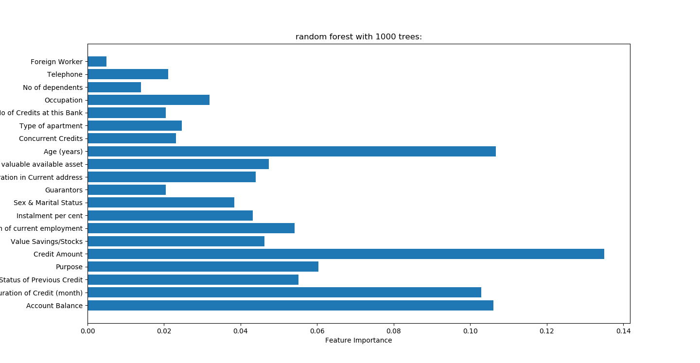
randomForest.py
random forest with 1000 trees:
accuracy on the training subset:1.000
accuracy on the test subset:0.772
准确性高于决策树
# -*- coding: utf-8 -*-
"""
Created on Sat Mar 31 09:30:24 2018

@author: Administrator
随机森林不需要预处理数据
"""
import pandas as pd
import numpy as np
import matplotlib.pyplot as plt
from sklearn.ensemble import RandomForestClassifier
from sklearn.model_selection import train_test_split

trees=1000
#读取文件
readFileName="German_credit.xlsx"

#读取excel
df=pd.read_excel(readFileName)
list_columns=list(df.columns[:-1])
X=df.ix[:,:-1]
y=df.ix[:,-1]
names=X.columns

x_train,x_test,y_train,y_test=train_test_split(X,y,random_state=0)
#n_estimators表示树的个数,测试中100颗树足够
forest=RandomForestClassifier(n_estimators=trees,random_state=0)
forest.fit(x_train,y_train)

print("random forest with %d trees:"%trees)
print("accuracy on the training subset:{:.3f}".format(forest.score(x_train,y_train)))
print("accuracy on the test subset:{:.3f}".format(forest.score(x_test,y_test)))
print('Feature importances:{}'.format(forest.feature_importances_))

n_features=X.shape[1]
plt.barh(range(n_features),forest.feature_importances_,align='center')
plt.yticks(np.arange(n_features),names)
plt.title("random forest with %d trees:"%trees)
plt.xlabel('Feature Importance')
plt.ylabel('Feature')
plt.show()
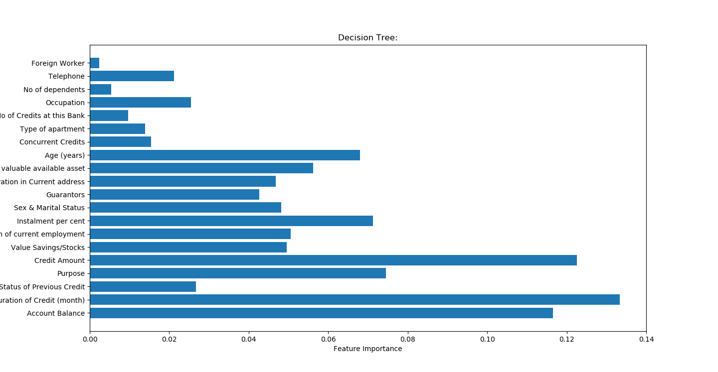
比较之前
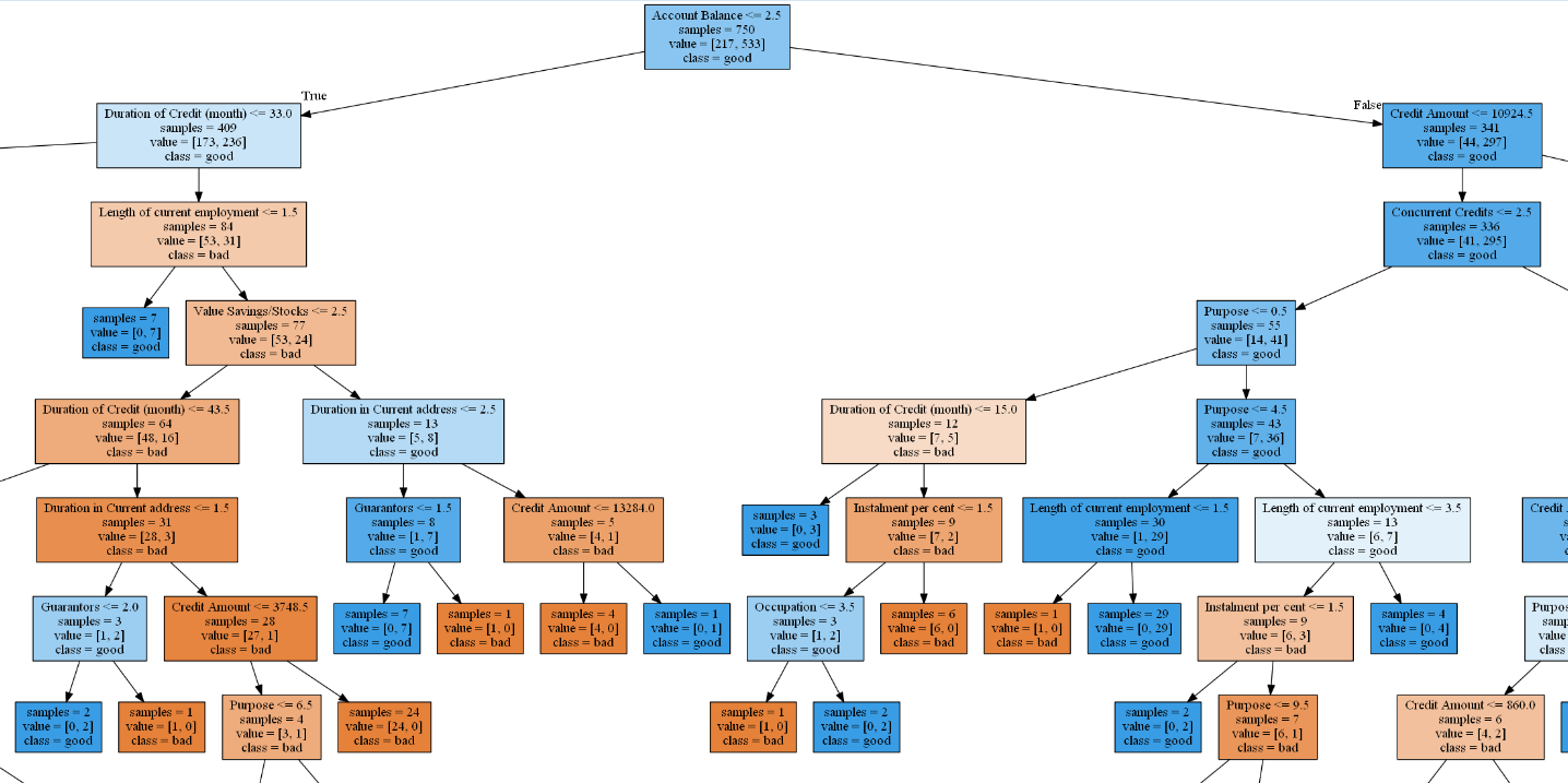
自己绘制树图
准确率不高,且严重过度拟合
accuracy on the training subset:0.991
accuracy on the test subset:0.680
# -*- coding: utf-8 -*-
"""
Created on Tue Apr 24 21:54:44 2018

@author: Administrator
"""

import pandas as pd
import numpy as np
import matplotlib.pyplot as plt
from sklearn.ensemble import RandomForestClassifier
import matplotlib.pyplot as plt
import numpy as np
import pydotplus
from IPython.display import Image
import graphviz
from sklearn.tree import export_graphviz
from sklearn.datasets import load_breast_cancer
from sklearn.tree import DecisionTreeClassifier
from sklearn.model_selection import train_test_split

trees=1000
#读取文件
readFileName="German_credit.xlsx"

#读取excel
df=pd.read_excel(readFileName)
list_columns=list(df.columns[:-1])
x=df.ix[:,:-1]
y=df.ix[:,-1]
names=x.columns

x_train,x_test,y_train,y_test=train_test_split(x,y,random_state=0)
#调参
list_average_accuracy=[]
depth=range(1,30)
for i in depth:
    #max_depth=4限制决策树深度可以降低算法复杂度,获取更精确值
    tree= DecisionTreeClassifier(max_depth=i,random_state=0)
    tree.fit(x_train,y_train)
    accuracy_training=tree.score(x_train,y_train)
    accuracy_test=tree.score(x_test,y_test)
    average_accuracy=(accuracy_training+accuracy_test)/2.0
    #print("average_accuracy:",average_accuracy)
    list_average_accuracy.append(average_accuracy)

max_value=max(list_average_accuracy)
#索引是0开头,结果要加1
best_depth=list_average_accuracy.index(max_value)+1
print("best_depth:",best_depth)

best_tree= DecisionTreeClassifier(max_depth=best_depth,random_state=0)
best_tree.fit(x_train,y_train)
accuracy_training=best_tree.score(x_train,y_train)
accuracy_test=best_tree.score(x_test,y_test)
print("decision tree:")
print("accuracy on the training subset:{:.3f}".format(best_tree.score(x_train,y_train)))
print("accuracy on the test subset:{:.3f}".format(best_tree.score(x_test,y_test)))

n_features=x.shape[1]
plt.barh(range(n_features),best_tree.feature_importances_,align='center')
plt.yticks(np.arange(n_features),names)
plt.title("Decision Tree:")
plt.xlabel('Feature Importance')
plt.ylabel('Feature')
plt.show()

#生成一个dot文件,以后用cmd形式生成图片
export_graphviz(best_tree,out_file="creditTree.dot",class_names=['bad','good'],feature_names=names,impurity=False,filled=True)


'''
best_depth: 12
decision tree:
accuracy on the training subset:0.991
accuracy on the test subset:0.680
'''
支持向量最高预测率
accuracy on the scaled training subset:0.867
accuracy on the scaled test subset:0.800
效果高于随机森林0.8-0.772=0.028
# -*- coding: utf-8 -*-
"""
Created on Fri Mar 30 21:57:29 2018

@author: Administrator
SVM需要标准化数据处理
"""
#标准化数据
from sklearn import preprocessing
from sklearn.svm import SVC
from sklearn.model_selection import train_test_split
import matplotlib.pyplot as plt
import pandas as pd

#读取文件
readFileName="German_credit.xlsx"

#读取excel
df=pd.read_excel(readFileName)
list_columns=list(df.columns[:-1])
x=df.ix[:,:-1]
y=df.ix[:,-1]
names=x.columns

#random_state 相当于随机数种子
X_train,x_test,y_train,y_test=train_test_split(x,y,stratify=y,random_state=42)
svm=SVC()
svm.fit(X_train,y_train)
print("accuracy on the training subset:{:.3f}".format(svm.score(X_train,y_train)))
print("accuracy on the test subset:{:.3f}".format(svm.score(x_test,y_test)))

'''
accuracy on the training subset:1.000
accuracy on the test subset:0.700

'''

#观察数据是否标准化
plt.plot(X_train.min(axis=0),'o',label='Min')
plt.plot(X_train.max(axis=0),'v',label='Max')
plt.xlabel('Feature Index')
plt.ylabel('Feature magnitude in log scale')
plt.yscale('log')
plt.legend(loc='upper right')

#标准化数据
X_train_scaled = preprocessing.scale(X_train)
x_test_scaled = preprocessing.scale(x_test)
svm1=SVC()
svm1.fit(X_train_scaled,y_train)
print("accuracy on the scaled training subset:{:.3f}".format(svm1.score(X_train_scaled,y_train)))
print("accuracy on the scaled test subset:{:.3f}".format(svm1.score(x_test_scaled,y_test)))
'''
accuracy on the scaled training subset:0.867
accuracy on the scaled test subset:0.800
'''


#改变C参数,调优,kernel表示核函数,用于平面转换,probability表示是否需要计算概率
svm2=SVC(C=10,gamma="auto",kernel='rbf',probability=True)
svm2.fit(X_train_scaled,y_train)
print("after c parameter=10,accuracy on the scaled training subset:{:.3f}".format(svm2.score(X_train_scaled,y_train)))
print("after c parameter=10,accuracy on the scaled test subset:{:.3f}".format(svm2.score(x_test_scaled,y_test)))
'''
after c parameter=10,accuracy on the scaled training subset:0.972
after c parameter=10,accuracy on the scaled test subset:0.716
'''


#计算样本点到分割超平面的函数距离
#print (svm2.decision_function(X_train_scaled))

#print (svm2.decision_function(X_train_scaled)[:20]>0)
#支持向量机分类
#print(svm2.classes_)

#malignant和bening概率计算,输出结果包括恶性概率和良性概率
#print(svm2.predict_proba(x_test_scaled))
#判断数据属于哪一类,0或1表示
#print(svm2.predict(x_test_scaled))
神经网络
效果不如支持向量和随机森林
最好概率
accuracy on the training subset:0.916
accuracy on the test subset:0.720

# -*- coding: utf-8 -*-
"""
Created on Sun Apr  1 11:49:50 2018

@author: Administrator
神经网络需要预处理数据
"""
#Multi-layer Perceptron 多层感知机
from sklearn.neural_network import MLPClassifier
#标准化数据,否则神经网络结果不准确,和SVM类似
from sklearn.preprocessing import StandardScaler
from sklearn.model_selection import train_test_split
import mglearn
import matplotlib.pyplot as plt
import numpy as np
import pandas as pd

#读取文件
readFileName="German_credit.xlsx"

#读取excel
df=pd.read_excel(readFileName)
list_columns=list(df.columns[:-1])
x=df.ix[:,:-1]
y=df.ix[:,-1]
names=x.columns

#random_state 相当于随机数种子
x_train,x_test,y_train,y_test=train_test_split(x,y,stratify=y,random_state=42)
mlp=MLPClassifier(random_state=42)
mlp.fit(x_train,y_train)
print("neural network:")
print("accuracy on the training subset:{:.3f}".format(mlp.score(x_train,y_train)))
print("accuracy on the test subset:{:.3f}".format(mlp.score(x_test,y_test)))

scaler=StandardScaler()
x_train_scaled=scaler.fit(x_train).transform(x_train)
x_test_scaled=scaler.fit(x_test).transform(x_test)

mlp_scaled=MLPClassifier(max_iter=1000,random_state=42)
mlp_scaled.fit(x_train_scaled,y_train)
print("neural network after scaled:")
print("accuracy on the training subset:{:.3f}".format(mlp_scaled.score(x_train_scaled,y_train)))
print("accuracy on the test subset:{:.3f}".format(mlp_scaled.score(x_test_scaled,y_test)))


mlp_scaled2=MLPClassifier(max_iter=1000,alpha=1,random_state=42)
mlp_scaled2.fit(x_train_scaled,y_train)
print("neural network after scaled and alpha change to 1:")
print("accuracy on the training subset:{:.3f}".format(mlp_scaled2.score(x_train_scaled,y_train)))
print("accuracy on the test subset:{:.3f}".format(mlp_scaled2.score(x_test_scaled,y_test)))


#绘制颜色图,热图
plt.figure(figsize=(20,5))
plt.imshow(mlp_scaled.coefs_[0],interpolation="None",cmap="GnBu")
plt.yticks(range(30),names)
plt.xlabel("columns in weight matrix")
plt.ylabel("input feature")
plt.colorbar()

'''
neural network:
accuracy on the training subset:0.700
accuracy on the test subset:0.700
neural network after scaled:
accuracy on the training subset:1.000
accuracy on the test subset:0.704
neural network after scaled and alpha change to 1:
accuracy on the training subset:0.916
accuracy on the test subset:0.720
'''