Unconstrained Optimization
3. Edition, March 2004
Poul Erik Frandsen, Kristian Jonasson Hans Bruun Nielsen, Ole Tingleff
2 Descent Methods
这里我们介绍的方法都是迭代方法。
对于求解函数的 局部极小值点 x*, 我们通过迭代产生一系列点,不断的逼近 x*
对于一个 stationary point 满足如下关系
但是这个点可能收敛于 a saddle point or even a maximizer。但是 descending property (2.2) 可以排除这些情况
误差应该是不断变小的
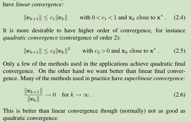
不同的方法具有不同的收敛速度,在迭代的过程中,收敛的速度很重要。
2.1. Fundamental Structure of a Descent Method
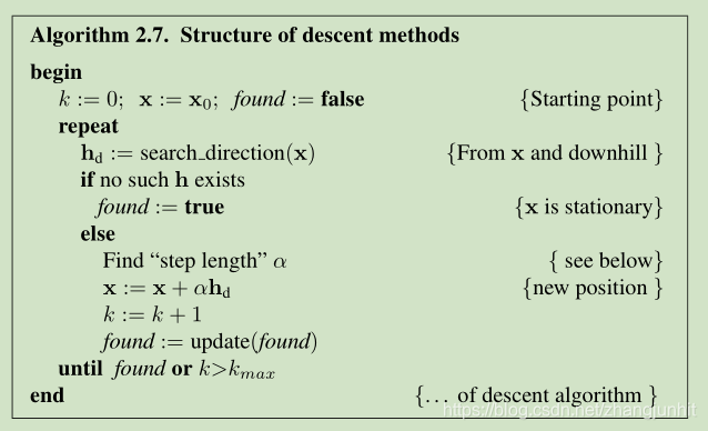
descent methods 主要包含两个步骤:1)方向的确定,2)步长的确定
算法迭代的 stopping criterion :这里我们介绍了几种迭代停止准则
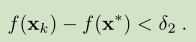
1) the current error is sufficiently small
2) the current value of f(x) is close enough to the minimal value
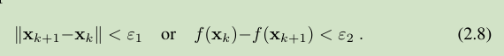
because x* and f(x*) are not known,所以我们比较前后两个向量的关系
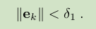
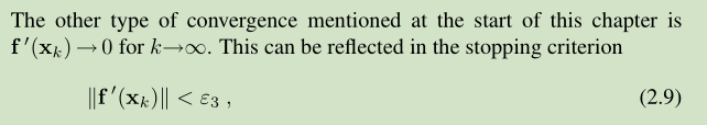
3) 还有一种收敛的描述以及对应的 停止迭代准则,因为在局部极小值位置,函数对应的一阶导数为 0,
所以收敛序列的一阶导数应该逼近 0
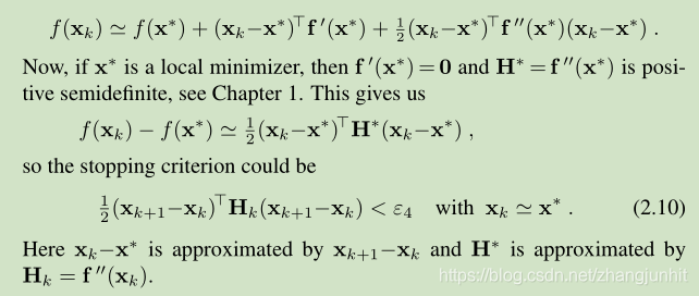
4) 在 x* 附近进行泰勒展开,根据局部极小值定义,我们可以得到另一个 stopping criterion 形式(2.10)
2.2. Descent Directions 下降方向
从当前位置 x 出发,我们希望找到一个方向,沿着它我们可以下山,该方向称之为 a descent direction。也就是说我们沿着该方向移动 a small step ( αh),我们得到一个更小的函数值: f(x+ αh)<f(x)
泰勒一阶展开如下
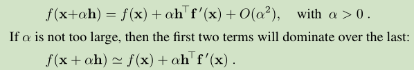
上面公式右边第二项 α h^T f’(x) 的正负号决定了我们是上山还是下山。
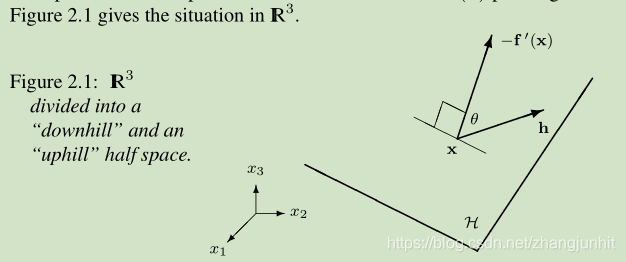
在n维 实数空间,我们定义一个 hyperplane H,它经过当前位置,垂直于 -f’(x)
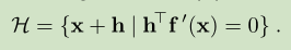
这个超平面将空间一分为二,一半空间对应 uphill,一半对应 downhill。 我们寻找的 一半空间:向量 -f’(x)指向 downhill 对应的半空间
接着我们定义 descent direction
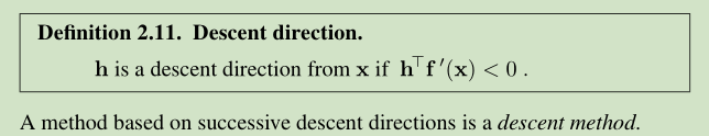
descent method 是基于 一系列 descent directions
根据 Figure 2.1 我们定义一个角 θ
the angle between h and -f’(x)
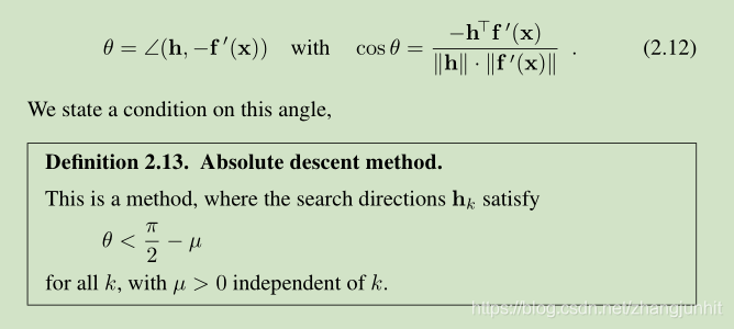
上面给出了绝对下降方法,该方法的 search directions h 与 -f’(x) 夹角 θ 小于 90度 大于 0
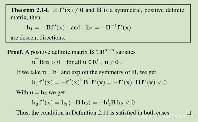
下面这个定理 描述了 -f’(x) 和 下降方向的关系
2.3. Descent Methods with Line Search
当我们确定了 descent direction,接下来我们就需要确定 沿着这个方向我们走多远了,步子迈的太大太小都不好。这里我们介绍 line search 的思路。这里我们来分析 目标函数 f 在当前位置沿着 h 其函数值的变化
ϕ(α) = f(x+αh), with fixed x and h 固定 x 和 h, 分析 α, 求解一个最优的 α, α>0
根据 (1.7)

ϕ(α) = f(x+αh) 的泰勒展开如下 ,这里的 α>0
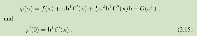
下图显示了一个 ϕ(α) 变化的实例,α>0, 所以只分析 y 轴的右侧。 ϕ(0) 这个位置算是起点,在该位置的 h 是一个 descent direction,方向是下降的,切线方向 右下倾。有了下降方向,我们需要寻找一个 α 值(沿着下降方向的移动步长)。
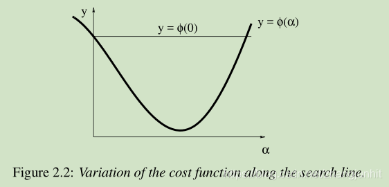
根据 descending condition (2.2),当我们找到一个值 αs 使得 ϕ(αs ) < ϕ(0),即实现了函数值的减小这个目标。那么我们应该停止 line search,因为已经完成任务了。但是上图所示,存在这样的风险:当 α 过大, 导致 ϕ(α) > ϕ(0),对应上图 ϕ(0) 右交点的右侧 α。 这个时候我们就要 减小 α 了。 还有一种特殊情况就是当 α 很小,导致函数值的变化基本消失了,这个时候我们需要增大 α。
下面我们使用公式来表达 防止这个 α 太大 太小问题。先上图
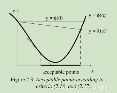
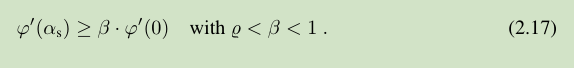
防止 α 太大 的 条件: gives a ϕ-value below that of the line y = λ(α), αs 需要在 直线 y = λ(α) 下方
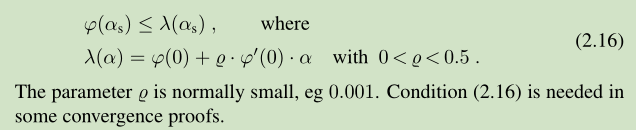
防止 α 太小 的 条件: ensuring that the local slope is greater than the starting slope. More specific,
Descent methods with line search governed by (2.16) and (2.17) are normally convergent
下面介绍一个相关的定理:
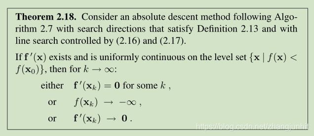
上面的下降方法收敛的结果分三种情况:1) 找到一个 stationary point,停止于位置 xk with f’(xk )=0;2)fall into the hole;3)收敛于一个 stationary point,通常这个stationary point 也是 a local minimizer
满足 (2.16) and (2.17) 的 line search 称之为 soft line search 。
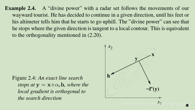
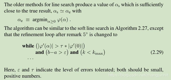
还有一种我们称之为 exact line search, when we seek (an approximation to) a local minimizer in the direction given by h
这里直接通过优化方法将 近似最优的 α 值 αe 求解出来。

αe 的一个必要条件是 ϕ’(αe )=0, 我们有 ϕ’(α) = h^T f’(x+αh), 这就对应两种情况:要么 f’(x+αe h)=0,要么 f’(x+αe h)!=0, f’(x+αe h)垂直于 h。
This shows that the exact line search will stop at a point where the local gradient is orthogonal to the search direction.
exact line search 停止于这里: 局部梯度和搜索方向垂直的点。
Sections 2.5 – 2.6 还会继续介绍 line search, 接下来介绍一些方法不依赖于 line search 来计算 step length
2.4. Descent Methods with Trust Region
本文描述的方法从起点开始产生一系列迭代收敛于最终结果,这是我们期望的。本章介绍的下降方法和第五章介绍的牛顿方法,步长的方向根据当前位置 f(x) 属性来确定。类似的考虑让我们得到 信赖域(Trust Region)方法,在该方法中,迭代步长由 目标函数在给定区域的模型属性决定。区域的尺寸在迭代过程是动态调整的。
Similar considerations lead us to the trust region methods, where the iteration steps are determined from the properties of a model of the objective function inside a given region. The size of the region is modified during the iteration.
在给定位置 x 的一阶泰勒展开为

二阶泰勒展开为
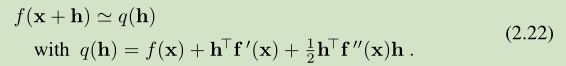
当||h||足够小,这两个 q(h) 都可以对 f(x+h) 较好的近似。迭代步长的确定可以用如下 model problem 来描述
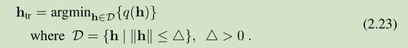
D 称之为 信赖域 trust region, q(h) 有 (2.21) or (2.22)表示。
我们使用 h=h_tr 作为一个下一步迭代的候选步长,如果 f(x+h)>f(x) ,我们就 reject h。损失函数的变化量决定了 信赖域的尺寸大小,对于下一步迭代来说。 这里我们定义 gain factor
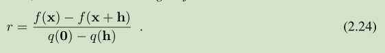
When r is small our approximation agrees poorly with f, when it is large the agreement is good
当 r 很小时,我们对 f 是近似比较差,当 r 较大时,我们的近似就比较好
所以我们通过 gain factor 来控制 trust region 的尺寸大小
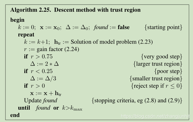
上面算法中的一些参数可以实际问题重新设定。
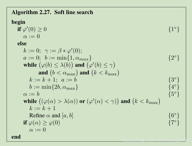
2.5. Soft Line Search
soft line search 的一个优势就是比 exact line search 要快。 exact line search 尽管可能迭代步数较少,但是每一步计算量要大于soft line search ,最终的结果往往是 soft line search 比 exact line search 要快
soft line search 另一个优势就是 它对起始点位置不太敏感。
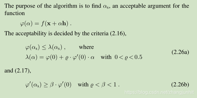
这两个 criteria 描述了 αs 不能太大也不能太小。
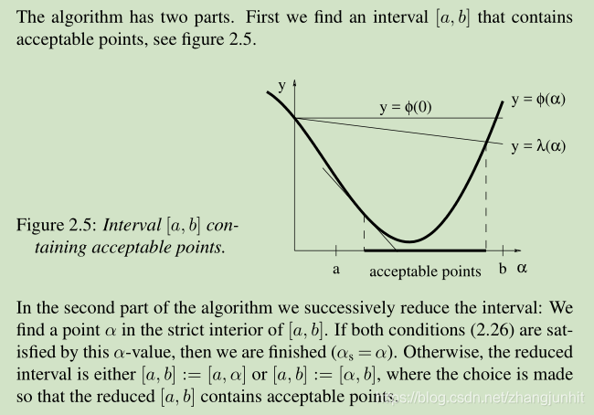
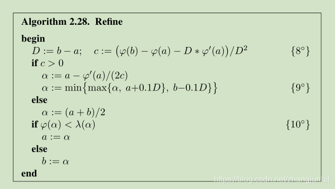
这个算法包含两个部分:1)找到一个 interval [a,b],包含可接受点。2)在 [a,b] 内部找到一个点 α
2.6. Exact Line Search
11