PyTorch基础入门四：PyTorch搭建逻辑回归模型进行分类

1）理论基础

Logistic起源于对人口数量增长情况的研究，后来又被应用到了对于微生物生长情况的研究，以及解决经济学相关的问题，现在作为一种回归分析的分支来处理分类问题。所以，虽然名字上听着是“回归”，但实际上处理的问题是“分类”问题。

先来看一下什么是Logistic分布吧。设 $X$ 是连续的随机变量，服从Logistic分布是指 $X$ 的积累分布函数和密度函数如下：

$F(x) = P(X\leqslant x) = \frac{1}{1+e^{-(x-\mu)/\gamma }}$

$f(x)=\frac{e^{-(x-\mu )/\gamma }}{\gamma (1+e^{-(x-\mu )/\gamma })^{2}}$

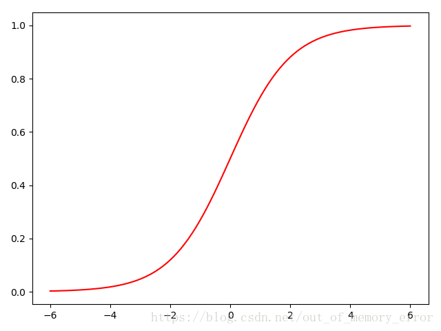
其中 $\mu$ 影响中心对称点的位置。 $\gamma$ 越小中心点附近增长越快。而在Logistic问题中，常用一种非线性变换的函数 $Sigmoid$ 函数来进行处理，这种函数其实就是分布函数 $\gamma =1$ ， $\mu =0$ 的特殊形式。其表达式如下：

$Sigmoid(x) = \frac{1}{1+e^{-x}}$

其图像如下：

现在了解了Logistic分布，接下来就看看它是如何处理二分类问题的吧。只要解决了二分类问题，其他分类问题都可以在二分类的基础之上进行建模。所以我们先来看看二分类问题吧。

假设输入的数据的特征向量 $x\in R^{n}$ ，那么决策边界可以表示为 $\sum_{i=1}^{n}w_{i}x_{i}+b=0$ ;假设存在一个样本使得 $h_{w}(x)=\sum_{i=1}^{n}w_{i}x_{i}+b>0$ ，那么可以判定它的类别是1；如果 $h_{w}(x)=\sum_{i=1}^{n}w_{i}x_{i}+b<0$ ，那么可以判定其类别是0.这个过程其实是一个感知机的过程，通过决策函数的符号来判断其属于哪一类。而Logistic回归要更进一步，通过找到分类概率：

$P(Y=0|x)=\frac{1}{1+e^{wx+b}}$

$P(Y=1|x)=\frac{e^{wx+b}}{1+e^{wx+b}}$

其中 $w$ 是权重， $b$ 是偏置。现在介绍Logistic模型的特点，先引入一个概念：一个事件发生的几率是指该事件发生的概率与不发生的概率的比值，比如一个事件发生的概率是 $p$ ，那么该时间发生的几率就是 $\frac{p}{1-p}$ ，该事件的对数几率或者logit函数是：

$logit(p)=log\frac{p}{1-p}$

对于Logistic回归而言，我们由之前的推导可以得到：

$log\frac{P(Y=1|x)}{1-P(Y=1|x)}=wx+b$

这也就是说在Logistic回归模型中，输出 $Y=1$ 的对数几率是输入 $x$ 的线性函数，这也就是Logisti回归名称的原因。简单的说，我们也可以这样定义Logistic回归：即线性函数的值越接近正无穷，概率值就越接近1；线性函数的值越接近负无穷，概率值就越接近0。因此Logistic回归的思路是先拟合决策边界（这里的决策边界不局限于线性，还可以是多项式等更为复杂的形式），在建立这个边界和分类概率的关系，从而得到二分类情况下的概率。

上面简单介绍了Logistic回归模型的建立，之后我们需要知道如何进行模型的参数估计。一般最常用的方式就是著名的梯度下降法。关于梯度下降的基本原理，这里不再赘述。

2）代码实现

首先我们依然需要“制造”出我们的假数据。当然这里的“假”是指这些数据没有实际意义，用来写实验性代码是完全没有任何顾虑的。代码如下：

# 假数据
n_data = torch.ones(100, 2)         # 数据的基本形态
x0 = torch.normal(2*n_data, 1)      # 类型0 x data (tensor), shape=(100, 2)
y0 = torch.zeros(100)               # 类型0 y data (tensor), shape=(100, 1)
x1 = torch.normal(-2*n_data, 1)     # 类型1 x data (tensor), shape=(100, 1)
y1 = torch.ones(100)                # 类型1 y data (tensor), shape=(100, 1)

# 注意 x, y 数据的数据形式是一定要像下面一样 (torch.cat 是在合并数据)
x = torch.cat((x0, x1), 0).type(torch.FloatTensor)  # FloatTensor = 32-bit floating
y = torch.cat((y0, y1), 0).type(torch.FloatTensor)    # LongTensor = 64-bit integer

# 画图
# plt.scatter(x.data.numpy()[:, 0], x.data.numpy()[:, 1], c=y.data.numpy(), s=100, lw=0, cmap='RdYlGn')
# plt.show()

上面的代码制造出的数据，输入两维，输出一维，可以方便的在平面上画出此数据的分布：

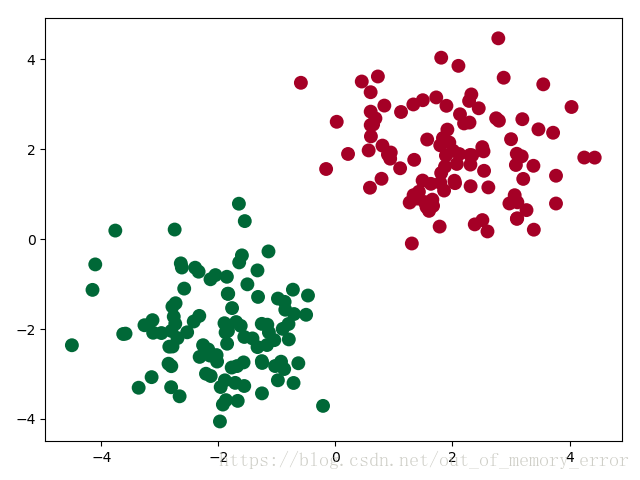
可以看到，上图中的点可以分类两类，我们就需要设计一个模型将其正确分类。

接下来我们定义Logistic回归模型，以及二分类问题的损失函数和优化器。需要值得注意的是，这里定义的损失函数为BCE存损失函数，有关BCE损失函数的详细描述，请参考：BCELoss。下面是代码部分：

class LogisticRegression(nn.Module):
    def __init__(self):
        super(LogisticRegression, self).__init__()
        self.lr = nn.Linear(2, 1)
        self.sm = nn.Sigmoid()

    def forward(self, x):
        x = self.lr(x)
        x = self.sm(x)
        return x

logistic_model = LogisticRegression()
if torch.cuda.is_available():
    logistic_model.cuda()

# 定义损失函数和优化器
criterion = nn.BCELoss()
optimizer = torch.optim.SGD(logistic_model.parameters(), lr=1e-3, momentum=0.9)

然后开始训练：

# 开始训练
for epoch in range(10000):
    if torch.cuda.is_available():
        x_data = Variable(x).cuda()
        y_data = Variable(y).cuda()
    else:
        x_data = Variable(x)
        y_data = Variable(y)

    out = logistic_model(x_data)
    loss = criterion(out, y_data)
    print_loss = loss.data.item()
    mask = out.ge(0.5).float()  # 以0.5为阈值进行分类
    correct = (mask == y_data).sum()  # 计算正确预测的样本个数
    acc = correct.item() / x_data.size(0)  # 计算精度
    optimizer.zero_grad()
    loss.backward()
    optimizer.step()
    # 每隔20轮打印一下当前的误差和精度
    if (epoch + 1) % 20 == 0:
        print('*'*10)
        print('epoch {}'.format(epoch+1)) # 训练轮数
        print('loss is {:.4f}'.format(print_loss))  # 误差
        print('acc is {:.4f}'.format(acc))  # 精度

根据前面几次博文的代码应该不难发现，在使用PyTorch定义和训练模型的过程中，有很多模板代码，这种模板代码由读者自己去体会。上述代码中有一行需要说明：mask = out.ge(0.5).float()。这行代码的意思是将结果大于0.5的归类为1，结果小于0.5的归类为0。通过这个来计算后面的精度。

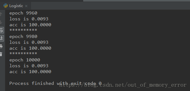
经过一万次的迭代，我们可以看到程序执行结果为：

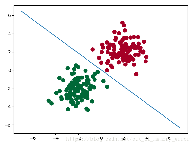
最后，我们把训练好的模型画出来，通过下面的图可以看出，已经将原始数据点完全的分为两类了。

附上完整代码：

# !/usr/bin/python
# coding: utf8
# @Time    : 2018-07-29 18:31
# @Author  : Liam
# @Email   : [email protected]
# @Software: PyCharm
#                        .::::.
#                      .::::::::.
#                     :::::::::::
#                  ..:::::::::::'
#               '::::::::::::'
#                 .::::::::::
#            '::::::::::::::..
#                 ..::::::::::::.
#               ``::::::::::::::::
#                ::::``:::::::::'        .:::.
#               ::::'   ':::::'       .::::::::.
#             .::::'      ::::     .:::::::'::::.
#            .:::'       :::::  .:::::::::' ':::::.
#           .::'        :::::.:::::::::'      ':::::.
#          .::'         ::::::::::::::'         ``::::.
#      ...:::           ::::::::::::'              ``::.
#     ```` ':.          ':::::::::'                  ::::..
#                        '.:::::'                    ':'````..
#                     美女保佑 永无BUG

import torch
from torch import nn
from torch.autograd import Variable
import matplotlib.pyplot as plt
import numpy as np

# 假数据
n_data = torch.ones(100, 2)         # 数据的基本形态
x0 = torch.normal(2*n_data, 1)      # 类型0 x data (tensor), shape=(100, 2)
y0 = torch.zeros(100)               # 类型0 y data (tensor), shape=(100, 1)
x1 = torch.normal(-2*n_data, 1)     # 类型1 x data (tensor), shape=(100, 1)
y1 = torch.ones(100)                # 类型1 y data (tensor), shape=(100, 1)

# 注意 x, y 数据的数据形式是一定要像下面一样 (torch.cat 是在合并数据)
x = torch.cat((x0, x1), 0).type(torch.FloatTensor)  # FloatTensor = 32-bit floating
y = torch.cat((y0, y1), 0).type(torch.FloatTensor)    # LongTensor = 64-bit integer

# 画图
# plt.scatter(x.data.numpy()[:, 0], x.data.numpy()[:, 1], c=y.data.numpy(), s=100, lw=0, cmap='RdYlGn')
# plt.show()

class LogisticRegression(nn.Module):
    def __init__(self):
        super(LogisticRegression, self).__init__()
        self.lr = nn.Linear(2, 1)
        self.sm = nn.Sigmoid()

    def forward(self, x):
        x = self.lr(x)
        x = self.sm(x)
        return x

logistic_model = LogisticRegression()
if torch.cuda.is_available():
    logistic_model.cuda()

# 定义损失函数和优化器
criterion = nn.BCELoss()
optimizer = torch.optim.SGD(logistic_model.parameters(), lr=1e-3, momentum=0.9)

# 开始训练
for epoch in range(10000):
    if torch.cuda.is_available():
        x_data = Variable(x).cuda()
        y_data = Variable(y).cuda()
    else:
        x_data = Variable(x)
        y_data = Variable(y)

    out = logistic_model(x_data)
    loss = criterion(out, y_data)
    print_loss = loss.data.item()
    mask = out.ge(0.5).float()  # 以0.5为阈值进行分类
    correct = (mask == y_data).sum()  # 计算正确预测的样本个数
    acc = correct.item() / x_data.size(0)  # 计算精度
    optimizer.zero_grad()
    loss.backward()
    optimizer.step()
    # 每隔20轮打印一下当前的误差和精度
    if (epoch + 1) % 20 == 0:
        print('*'*10)
        print('epoch {}'.format(epoch+1)) # 训练轮数
        print('loss is {:.4f}'.format(print_loss))  # 误差
        print('acc is {:.4f}'.format(acc))  # 精度

# 结果可视化
w0, w1 = logistic_model.lr.weight[0]
w0 = float(w0.item())
w1 = float(w1.item())
b = float(logistic_model.lr.bias.item())
plot_x = np.arange(-7, 7, 0.1)
plot_y = (-w0 * plot_x - b) / w1
plt.scatter(x.data.numpy()[:, 0], x.data.numpy()[:, 1], c=y.data.numpy(), s=100, lw=0, cmap='RdYlGn')
plt.plot(plot_x, plot_y)
plt.show()