第三十四周学习笔记

CS231n

Visualizing and Understanding

可视化第一层
在这里插入图片描述
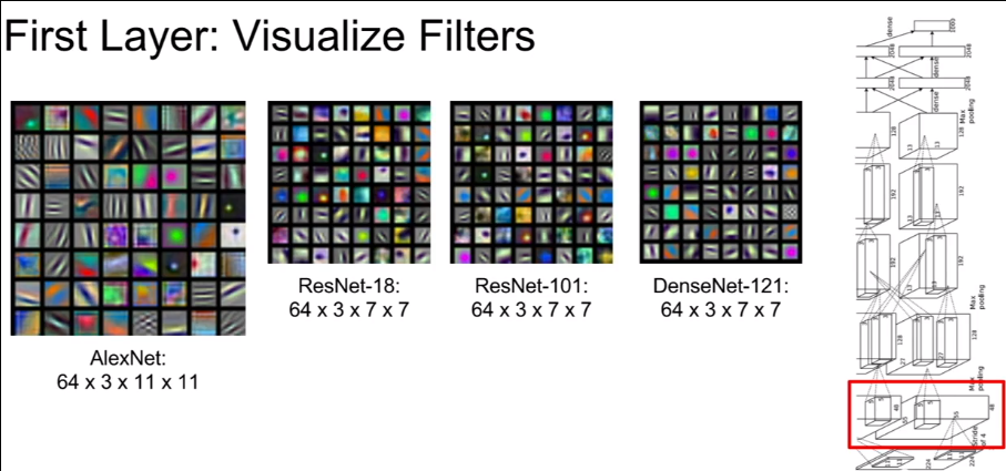
通过visualize卷积核，可以得到卷积核寻找的pattern，因为图像的局部与卷积核越接近，内积越大，激活图的值就越大

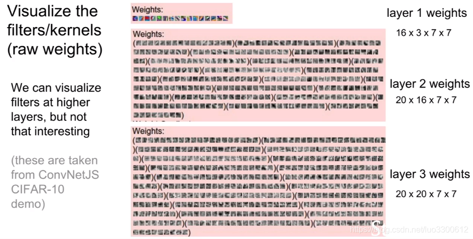
可视化第二层

第二层的可视化不如第一层那么简单直接，因为，第二层的卷积核维度很大，且不与输入直接关联
在这里插入图片描述
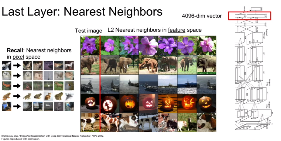
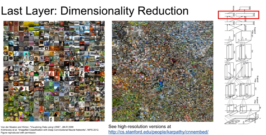
可视化最后一层
最后一层的可视化，将不同图片最后一层的输出向量用k-近邻或者降维方法（PCA、t-SNE）来可视化

可视化最大激活
在这里插入图片描述
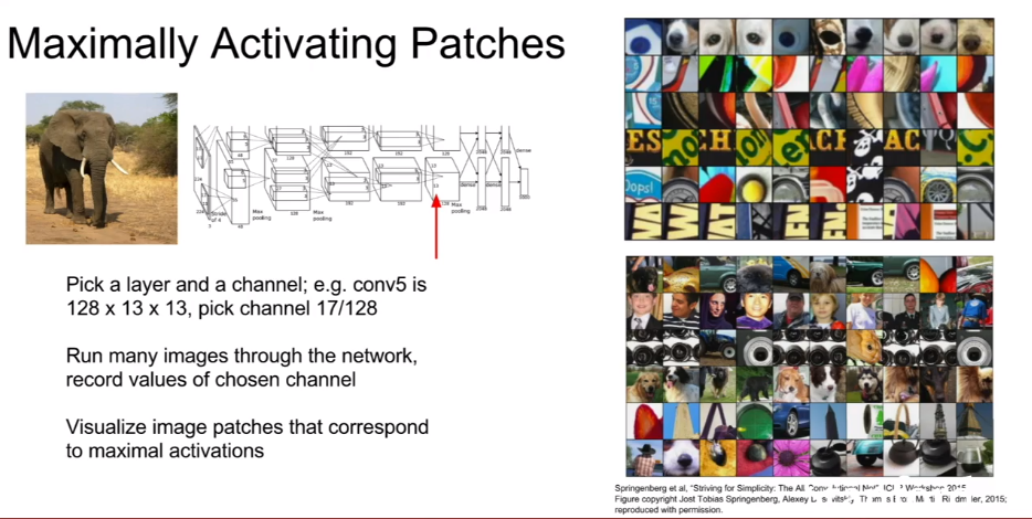
选择卷积层中的一个神经元（这里指的是一个channel上的所有共享权值的神经元），输入图片后，找到对应这个channel上激活最大的局部输入图片，从而发现该神经元所寻找的特征

Occlusion Experiments
在这里插入图片描述
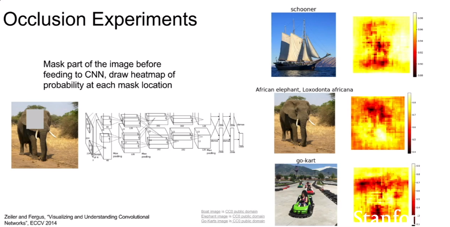
通过在图片上加mask的方法，找到与图片类别得分相关高的区域并画出热力图，从而得知网络分类所关心的特征

Saliency Maps
在这里插入图片描述
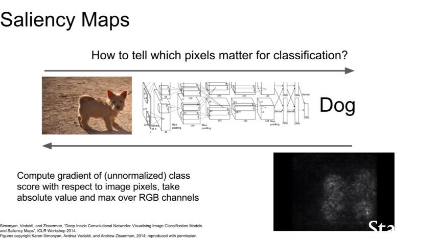
对输入求导，从而得知哪些像素对得分的影响大

优化图片
在这里插入图片描述
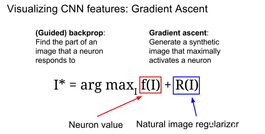
通过梯度下降来得到使得某类得分高的图片，使用正则化项防止生成图片过拟合而导致图片看起来是噪声

对抗样本
在这里插入图片描述
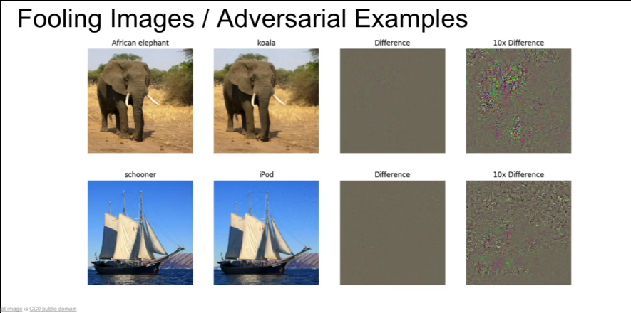
给一张大象的图片，让网络将其转化为类别为考拉的图片（可以通过之前对输入的梯度下降做到），最终得到一张在人眼看来没有区别，却被网络识别为考拉的图片

为什么要研究网络的可视化？
Justin：This whole field of trying to visualize intermediates is kind of in response to a common criticism of deep learning. So a common criticism of deep learning is like, you’ve got this big black box network, you trained it on gradient ascent, you get a good number and that’s great but we don’t trust the network because we don’t understand as people why it’s making the decisions, that’s it’s making. So a lot of these type of visualization techniques were developed to try and address that and try to understand as people why the network are making their various classification, classification decisions a bit more. Because if you contrast a deep convolutional neural network with other machine running techniques. Like linear models are much easier to interpret in general, because you can look at the weights and kind of understand the interpretation between how much each input feature effect the decision or if you look at something like a random forest or decision tree Some other machine learning models end up being a bit more interpretable just by their very nature than this sort of black box convolutional networks. So a lot of this is sort of in response to that criticism to say that yes they are these large complex models but they are still doing some interesting and interpretable thins under the hood. They are not just totally going out in randomly classifying things. They are doing something meaningful.

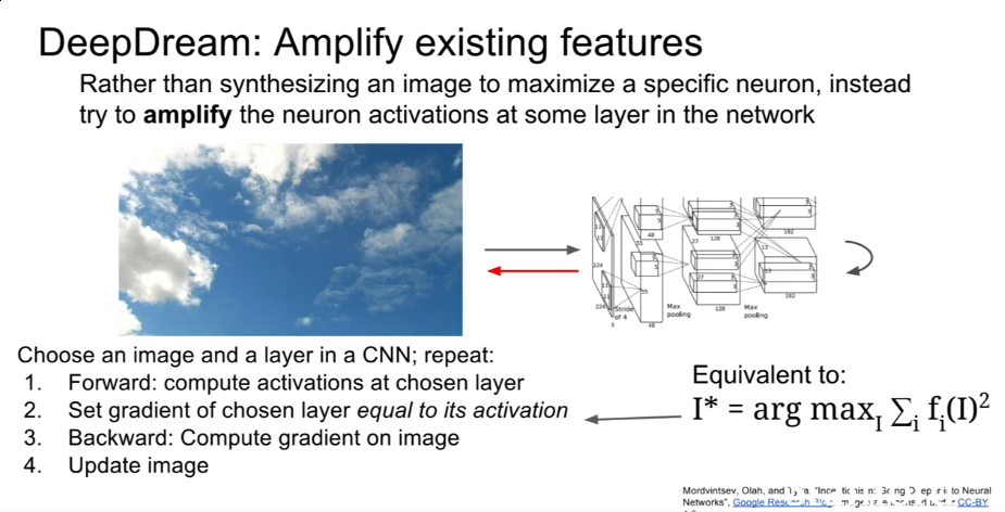
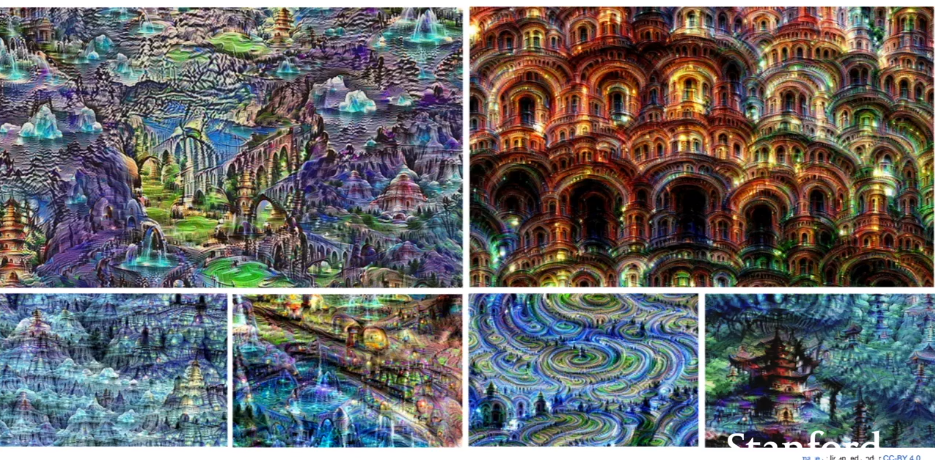
增强特征
在这里插入图片描述

在这里插入图片描述

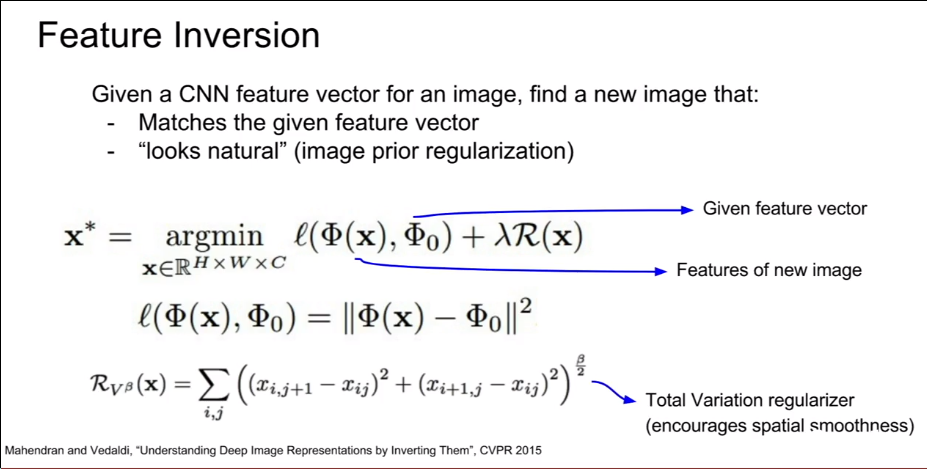
特征转化
在这里插入图片描述

风格迁移
在这里插入图片描述
最小化两张图片的特征向量距离实现风格迁移

总结

激活：最近邻、降维、最大patch、occlusion
梯度：Saliency maps，class visulization，fooling images，feature inversion
Fun：DeepDream，Style Transfer

Generative Models

Unsupervised Learning

supervised learning
数据：(x,y)，x是数据，y是标签
目标：学习一个映射x->y
例子：

分类
回归
目标检测
语义分割
image captioning

Unsupervised Learning
数据：x，只有数据，没有标签
目标：学习数据的隐含结构
例子：

聚类
降维
特征学习
密度估计（估计样本的分布）

Generative Models

生成模型在训练数据的基础上，目标是从相同的分布中生成新的样本，使得 $p_{model}(x)$ 和 $p_{data}(x)$ 相同，重点是密度估计（density estimation），可以是：

直接密度估计（explicit density estimation）：精确地定义并解出 $p_{model}(x)$
间接密度估计（implicit density estimation）：学习可以从 $p_{model}(x)$ 中采样的模型，而不精确定义它

Why Generative Models?

AI绘画、超分辨率、自动上色
时间序列的生成模型可以用来做模拟和规划（针对强化学习应用）
训练生成模型可以获得好的特征表示

在这里插入图片描述

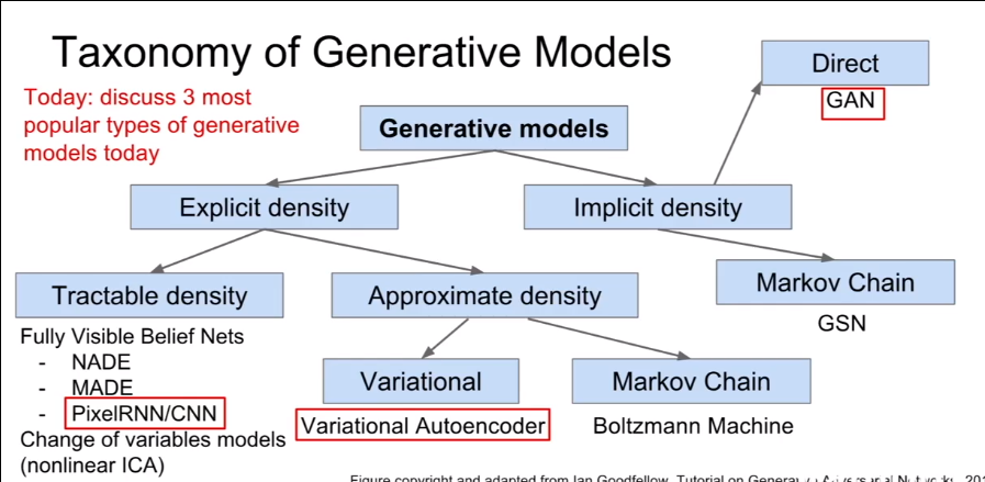
PixelRNN and PixelCNN

Fully visible belief network

精确的密度模型，使用链式法则将图片x的似然分解成一维分布的乘积：
$p(x)=\prod_{i=1}^{n}p(x_i|x_1,...,x_{i-1})$
其中需要定义像素的顺序，然后最大化训练数据的似然

PixelRNN

从角落开生成图片，使用RNN（LSTM）
缺点：使用序列生成很慢

PixelCNN

也从角落开始生成图片，在一个上下文区域中使用CNN
比PixelRNN块，但因为是序列处理的，所以还是很慢

PixelRNN 和 PixelCNN

优点：

可以精确给出似然p(x)
训练数据精确的似然可以给出好的度量矩阵
好的样例
缺点：
序列生成很慢

变分自编码器

PixelCNN定义易处理的密度函数，来最大化似然：
$p(x)=\prod_{i=1}^{n}p(x_i|x_1,...,x_{i-1})$

VAEs定义难处理的密度函数，使用隐变量z：
$p_\theta(x)=\int p_\theta(z)p_\theta(x|z)dz$
不能直接优化，只能优化似然的下界

在这里插入图片描述
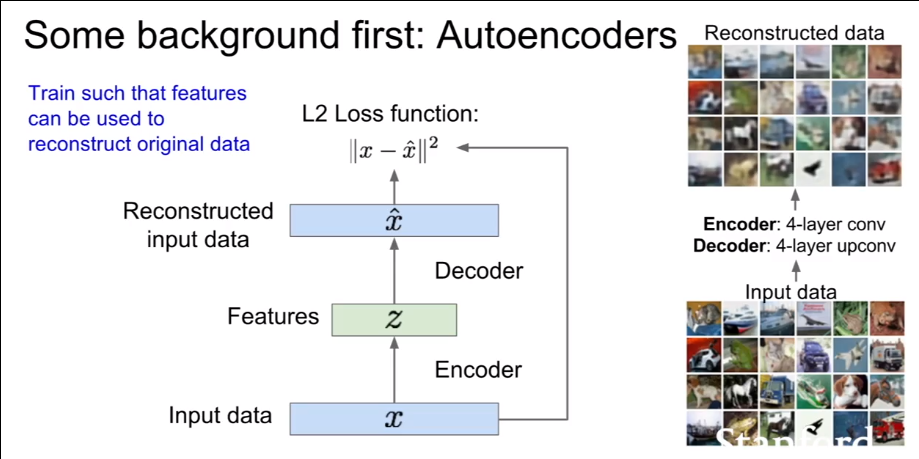
通过encoder将数据编码成低位隐变量z，然后用Decoder将隐变量重建为原图像，以重建误差为loss

生成图片时，先采样隐变量z，然后从条件分布 $p(x|z)$ 中抽样x

GANs

从简单的分布（例如随机噪声）中采样，学习它到训练分布的映射
训练GANs就是一个二人博弈游戏
Generator network：使用生成样本欺骗discriminator
discriminator network：区分真实和生成的图片

优点：

state-of-the-art的模型

缺点：

训练不稳定
不能解出p(x)和p(z|x)

Efficient Methods and Hardware for Deep Learning

Algorithms for Efficient Inference

Pruning，剪枝，将小的权值单元剪掉
权值共享，对权值进行聚类，然后将接近的权值用消耗内存更小的数值代替（比如2.01、2.04、1.97、1.99用2代替）
Quantization，使用float训练网络，然后通过权值和激活的统计信息，选择合适的小数点位置，然后在float格式下微调，最后转化为fixed-point格式
Binary/Ternary Net，使用两个或三个权值（比如-1，0，1）来代表一个神经网络
Winograd Transformation，对数据进行转化来减低复杂度

在这里插入图片描述

Hardware for Efficient Inference

在这里插入图片描述

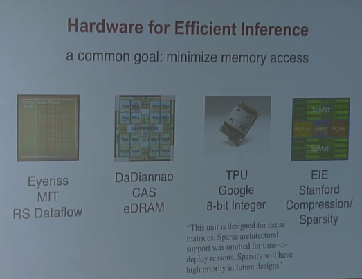
Google TPU

核心是一个大的矩阵乘法单元，一次循环中可以进行64k次乘法和累加操作，大约比GPU快25倍，比CPU快100倍

EIE：the First DNN Accelerator for Sparse, Compressed Model

sparse weight
sparse activation
weight sharing

在这里插入图片描述
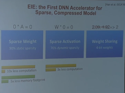
以CPU的速度为1-3x，GPU的速度就是15-48x，EIE的速度为189x

以CPU的能量效率为1-6x，GPU的效率为7-23x，EIE的效率为24207x…

Algorithms for Efficient training

Parallelization，矩阵乘法的并行，特征图的并行，不同超参数模型的并行
Mixed Precision with FP16 and FP32，在训练的不同时间使用不同的精度（比如前向传播的时候使用16bit的数值，权值更新的时候使用32bit的数值）
Model Distillation，使用高级的模型得到软化的label（比如[0.1,0.3,0.6]）来训练student model，而不是使用hard label（比如[1,0,0]）来训练
DSD：Dense Sparse Dense Training，先训练剪枝模型，然后继续训练原模型，类似于先张出树干，然后长出叶子的感觉

Hardware for Efficient training

GPU:

Kepler
Maxwell
Pascal
Volta

Google Cloud TPU

Future

smart
low latency
privacy
mobility
energy-efficient

Adversarial Examples and Adversarial Training

Adversarial Examples

对抗样本在人眼看来一样，却可以欺骗神经网络等几乎所有机器学习算法（线性回归、决策树等等）
在这里插入图片描述
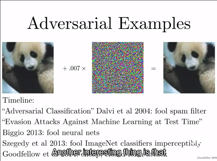
学习对抗样本能加深对当前模型的理解，并引出更好的模型

Adversarial Traning

神经网络可以通过Adversarial Training 变得更安全，相对于其他极其学习算法而言

Conclusion

attacking is easy
defending is difficult
adversarial training 提供正则化和半监督学习
out-of-domain的输入是基于模型优化的瓶颈

本周反思

阅读resnet的论文，未完成
继续完成cs231n的学习进度到100%，完成
学习opencv上册到50%，未完成

下周目标

阅读resnet的论文
学习opencv上册到50%
训练出初始的superpoint模型