综述

“余既滋兰之九畹兮，又树蕙之百亩”

本文采用编译器：jupyter

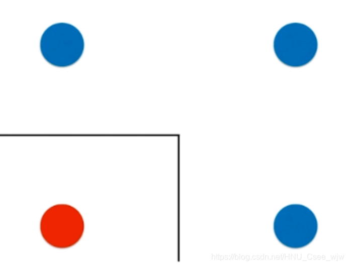
决策树 (decision tree) 是一类常见的机器学习方法，顾名思义，决策树是基于树结构来进行决策的，这恰是人类在面临决策问题时一种很自然的处理机制。

例如，我们要对“是否录用他作为机器学习算法工程师？”这样的问题进行决策时，通常会进行一系列的判断或“子决策”：我们先看“他是否发表过顶会论文？”如果是“没有”，则再看“是否是研究生？”如果是“是研究生”，再判断“他的项目是否和机器学习相关？”......最终我们得出决策。过程如图：

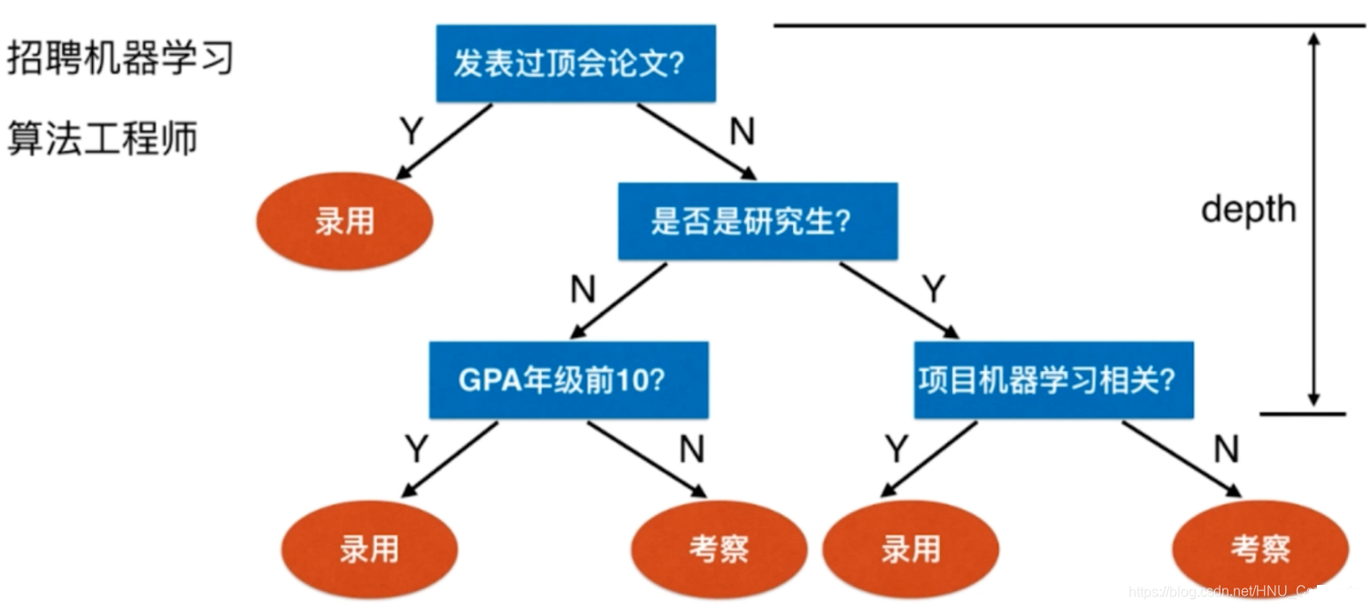
很明显，决策树是一种非参数学习算法，天然的可以解决多分类问题（也可以解决回归问题），并且得到的结果具有非常好的可解释性。

01 scikit-learn中的决策树

import numpy as np
import matplotlib.pyplot as plt

from sklearn import datasets

iris = datasets.load_iris()
X = iris.data[:,2:] # 取后两个特征
y = iris.target

plt.scatter(X[y==0,0], X[y==0,1])
plt.scatter(X[y==1,0], X[y==1,1])
plt.scatter(X[y==2,0], X[y==2,1])
plt.show()

from sklearn.tree import DecisionTreeClassifier

dt_clf = DecisionTreeClassifier(max_depth=2, criterion="entropy")
dt_clf.fit(X, y)
"""
Out[4]:
DecisionTreeClassifier(class_weight=None, criterion='entropy', max_depth=2,
            max_features=None, max_leaf_nodes=None,
            min_impurity_decrease=0.0, min_impurity_split=None,
            min_samples_leaf=1, min_samples_split=2,
            min_weight_fraction_leaf=0.0, presort=False, random_state=None,
            splitter='best')
"""

def plot_decision_boundary(model, axis):
    
    x0, x1 = np.meshgrid(
        np.linspace(axis[0], axis[1], int((axis[1]-axis[0])*100)).reshape(-1,1),
        np.linspace(axis[2], axis[3], int((axis[3]-axis[2])*100)).reshape(-1,1)
    )
    X_new = np.c_[x0.ravel(), x1.ravel()]
    
    y_predict = model.predict(X_new)
    zz = y_predict.reshape(x0.shape)
    
    from matplotlib.colors import ListedColormap
    custom_cmap = ListedColormap(['#EF9A9A', '#FFF59D','#90CAF9'])
    
    plt.contourf(x0, x1, zz, linewidth=5, cmap=custom_cmap)

plot_decision_boundary(dt_clf, axis=[0.5, 7.5, 0, 3])
plt.scatter(X[y==0,0], X[y==0,1])
plt.scatter(X[y==1,0], X[y==1,1])
plt.scatter(X[y==2,0], X[y==2,1])
plt.show()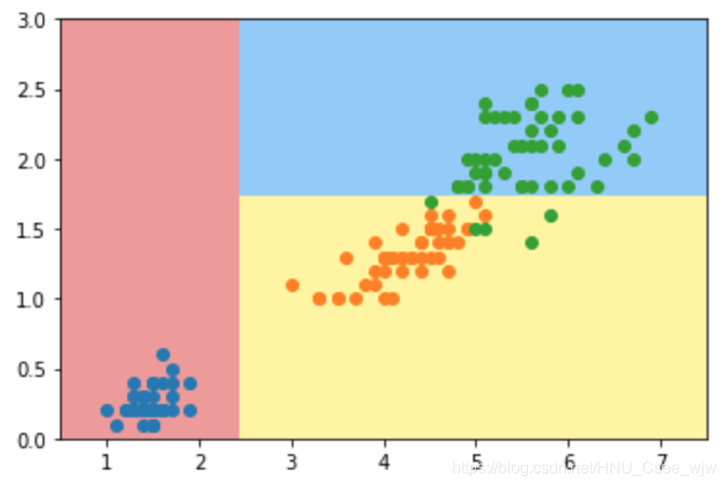

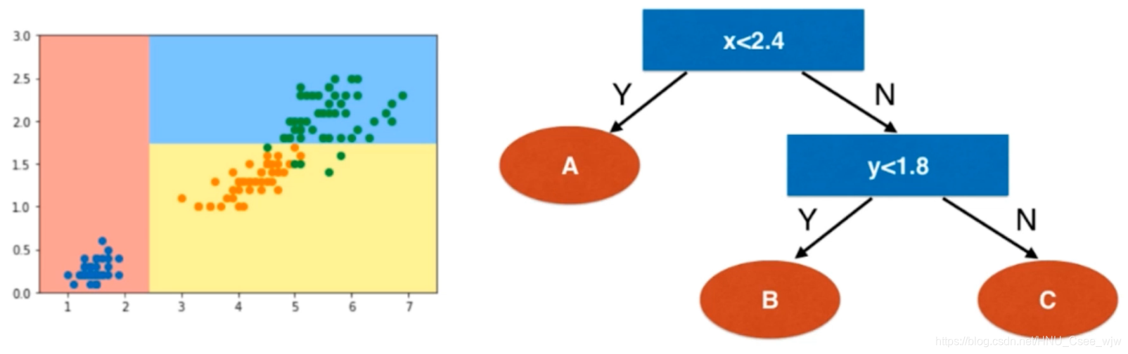
我们的到的决策树如下：

02 信息熵

经过简单的实践时候我们应该好奇构造一颗决策树的方法，即每个节点在哪个维度上做划分？以及某个维度在哪个值上做划分？

决策树中最常用的标准之一是信息熵，信息熵表示的是随机变量不确定度的度量。熵越大，数据的不确定性越高；熵越小，数据的不确定性越低。表达式如下：

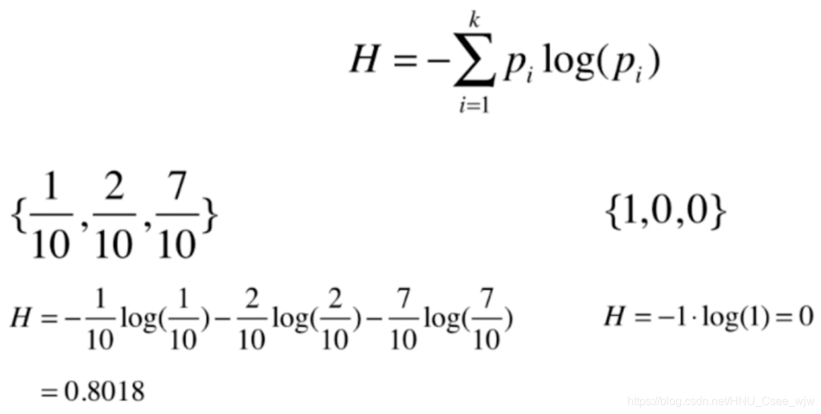
对于二分类任务：

所以对于上面提出的两个问题，我们的目的是使得划分后的信息熵降低

import numpy as np
import matplotlib.pyplot as plt

def entropy(p):
    return -p * np.log(p) - (1-p) * np.log(1-p)

x = np.linspace(0.01, 0.99, 200)

plt.plot(x, entropy(x))
plt.show()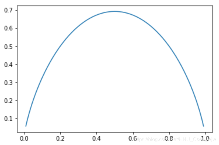

03 使用信息熵寻找最优划分

import numpy as np
import matplotlib.pyplot as plt

from sklearn import datasets

iris = datasets.load_iris()
X = iris.data[:,2:] # 取后两个特征
y = iris.target

from sklearn.tree import DecisionTreeClassifier

dt_clf = DecisionTreeClassifier(max_depth=2, criterion="entropy")
dt_clf.fit(X, y)
"""
Out[4]:
DecisionTreeClassifier(class_weight=None, criterion='entropy', max_depth=2,
            max_features=None, max_leaf_nodes=None,
            min_impurity_decrease=0.0, min_impurity_split=None,
            min_samples_leaf=1, min_samples_split=2,
            min_weight_fraction_leaf=0.0, presort=False, random_state=None,
            splitter='best')
"""

def plot_decision_boundary(model, axis):
    
    x0, x1 = np.meshgrid(
        np.linspace(axis[0], axis[1], int((axis[1]-axis[0])*100)).reshape(-1,1),
        np.linspace(axis[2], axis[3], int((axis[3]-axis[2])*100)).reshape(-1,1)
    )
    X_new = np.c_[x0.ravel(), x1.ravel()]
    
    y_predict = model.predict(X_new)
    zz = y_predict.reshape(x0.shape)
    
    from matplotlib.colors import ListedColormap
    custom_cmap = ListedColormap(['#EF9A9A', '#FFF59D','#90CAF9'])
    
    plt.contourf(x0, x1, zz, linewidth=5, cmap=custom_cmap)

plot_decision_boundary(dt_clf, axis=[0.5, 7.5, 0, 3])
plt.scatter(X[y==0,0], X[y==0,1])
plt.scatter(X[y==1,0], X[y==1,1])
plt.scatter(X[y==2,0], X[y==2,1])
plt.show()

模拟使用信息熵进行划分

# d:维度  value:阈值
def split(X, y, d, value):
    index_a = (X[:,d] <= value)
    index_b = (X[:,d] > value)
    return X[index_a], X[index_b], y[index_a], y[index_b]

# 计算阈值
from collections import Counter
from math import log

def entropy(y):
    counter = Counter(y) # 包装成字典
    res = 0.0
    for num in counter.values():
        p = num / len(y)
        res += -p * log(p)
    return res

def try_split(X, y):
    
    best_entropy = float('inf')
    best_d, best_v = -1, -1
    # 寻找用来划分用的的维度和阈值
    # 阈值取相邻大小两个点的中间值
    for d in range(X.shape[1]):
        sorted_index = np.argsort(X[:,d])
        # 对每个样本遍历
        for i in range(1, len(X)):
            if X[sorted_index[i-1], d] != X[sorted_index[i], d]:
                v = (X[sorted_index[i-1], d] + X[sorted_index[i], d]) / 2
                # 按照此维度与阈值进行划分
                X_l, X_r, y_l, y_r = split(X, y, d, v)
                # 计算信息熵
                e = entropy(y_l) + entropy(y_r)
                if e < best_entropy:
                    best_entropy, best_d, best_v = e, d, v
    
    return best_entropy, best_d, best_v
            
best_entropy, best_d, best_v = try_split(X, y)
print("best_entropy = ", best_entropy)
print("best_d = ", best_d)
print("best_v = ", best_v)
# 对比之前的边界图像可以看出，第一个划分的位置就是在横轴2.45附近
best_entropy =  0.6931471805599453
best_d =  0
best_v =  2.45

X1_l, X1_r, y1_l, y1_r = split(X, y, best_d, best_v)

entropy(y1_l) # 第一次划分成功把一个数据划分出来
# Out[14]:
# 0.0

entropy(y1_r)
# Out[15]:
# 0.6931471805599453

best_entropy2, best_d2, best_v2 = try_split(X1_r, y1_r)
print("best_entropy2 = ", best_entropy2)
print("best_d2 = ", best_d2)
print("best_v2 = ", best_v2)
# 对比之前的边界图像可以看出，第二个划分的位置就是在y轴1.75附近
best_entropy2 =  0.4132278899361904
best_d2 =  1
best_v2 =  1.75

X2_l, X2_r, y2_l, y2_r = split(X1_r, y1_r, best_d2, best_v2)

entropy(y2_l)
# Out[19]:
# 0.30849545083110386

entropy(y2_r)
# Out[20]:
# 0.10473243910508653

# 可以继续往更深的地方划分......

04 基尼系数

除了信息熵之外，还有另一种划分的标准，称为基尼系数。

和信息熵相比，大多时候二者没有特别的效果优劣，scikit-learn中默认为基尼系数。

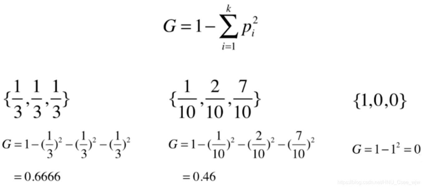
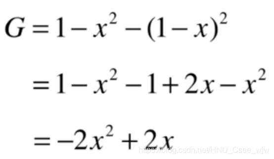
对于二分类问题：

import numpy as np
import matplotlib.pyplot as plt

from sklearn import datasets

iris = datasets.load_iris()
X = iris.data[:,2:] # 取后两个特征
y = iris.target

from sklearn.tree import DecisionTreeClassifier

dt_clf = DecisionTreeClassifier(max_depth=2, criterion="gini")
dt_clf.fit(X, y)
"""
Out[3]:
DecisionTreeClassifier(class_weight=None, criterion='gini', max_depth=2,
            max_features=None, max_leaf_nodes=None,
            min_impurity_decrease=0.0, min_impurity_split=None,
            min_samples_leaf=1, min_samples_split=2,
            min_weight_fraction_leaf=0.0, presort=False, random_state=None,
            splitter='best')
"""

def plot_decision_boundary(model, axis):
    
    x0, x1 = np.meshgrid(
        np.linspace(axis[0], axis[1], int((axis[1]-axis[0])*100)).reshape(-1,1),
        np.linspace(axis[2], axis[3], int((axis[3]-axis[2])*100)).reshape(-1,1)
    )
    X_new = np.c_[x0.ravel(), x1.ravel()]
    
    y_predict = model.predict(X_new)
    zz = y_predict.reshape(x0.shape)
    
    from matplotlib.colors import ListedColormap
    custom_cmap = ListedColormap(['#EF9A9A', '#FFF59D','#90CAF9'])
    
    plt.contourf(x0, x1, zz, linewidth=5, cmap=custom_cmap)

plot_decision_boundary(dt_clf, axis=[0.5, 7.5, 0, 3])
plt.scatter(X[y==0,0], X[y==0,1])
plt.scatter(X[y==1,0], X[y==1,1])
plt.scatter(X[y==2,0], X[y==2,1])
plt.show()
# 与信息熵得出的结果是相同的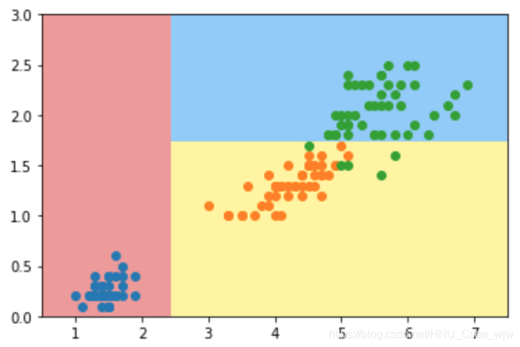

模拟使用基尼系数划分

from collections import Counter
from math import log

def split(X, y, d, value):
    index_a = (X[:,d] <= value)
    index_b = (X[:,d] > value)
    return X[index_a], X[index_b], y[index_a], y[index_b]

def gini(y):
    counter = Counter(y)
    res = 1.0
    for num in counter.values():
        p = num / len(y)
        res -= p**2
    return res

def try_split(X, y):
    
    best_g = 1e9
    best_d, best_v = -1, -1
    # 寻找用来划分用的的维度和阈值
    # 阈值取相邻大小两个点的中间值
    for d in range(X.shape[1]):
        sorted_index = np.argsort(X[:,d])
        # 对每个样本遍历
        for i in range(1, len(X)):
            if X[sorted_index[i-1], d] != X[sorted_index[i], d]:
                v = (X[sorted_index[i-1], d] + X[sorted_index[i], d]) / 2
                # 按照此维度与阈值进行划分
                X_l, X_r, y_l, y_r = split(X, y, d, v)
                # 计算信息熵
                g = gini(y_l) + gini(y_r)
                if g < best_g:
                    best_g, best_d, best_v = g, d, v
    
    return best_g, best_d, best_v

best_g, best_d, best_v = try_split(X, y)
print("best_g = ", best_g)
print("best_d = ", best_d)
print("best_v = ", best_v)
best_g =  0.5
best_d =  0
best_v =  2.45

X1_l, X1_r, y1_l, y1_r = split(X, y, best_d, best_v)
gini(y1_l) # 第一次划分成功把一个数据划分出来
# Out[9]:
# 0.0

gini(y1_r)
# Out[10]:
# 0.5

best_g2, best_d2, best_v2 =  try_split(X1_r, y1_r)
print("best_g2 = ", best_g2)
print("best_d2 = ", best_d2)
print("best_v2 = ", best_v2)
best_g2 =  0.2105714900645938
best_d2 =  1
best_v2 =  1.75

X2_l, X2_r, y2_l, y2_r = split(X1_r, y1_r, best_d2, best_v2)
gini(y2_l)
# Out[13]:
# 0.1680384087791495

gini(y2_r)
# Out[14]:
# 0.04253308128544431

05 CART和决策树的超参数

决策树复杂度分析：

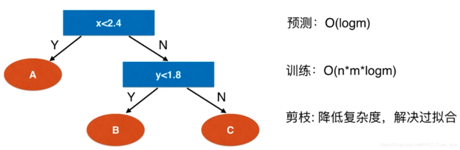
可以通过设置决策树的CART参数来降低复杂度。

import numpy as np
import matplotlib.pyplot as plt

from sklearn import datasets

X, y = datasets.make_moons()

X, y = datasets.make_moons(noise=0.25, random_state=666)

plt.scatter(X[y==0,0], X[y==0,1])
plt.scatter(X[y==1,0], X[y==1,1])
plt.show()

from sklearn.tree import DecisionTreeClassifier

dt_clf = DecisionTreeClassifier() # 划分标准默认为基尼系数
dt_clf.fit(X, y)
"""
Out[6]:
DecisionTreeClassifier(class_weight=None, criterion='gini', max_depth=None,
            max_features=None, max_leaf_nodes=None,
            min_impurity_decrease=0.0, min_impurity_split=None,
            min_samples_leaf=1, min_samples_split=2,
            min_weight_fraction_leaf=0.0, presort=False, random_state=None,
            splitter='best')
"""

def plot_decision_boundary(model, axis):
    
    x0, x1 = np.meshgrid(
        np.linspace(axis[0], axis[1], int((axis[1]-axis[0])*100)).reshape(-1,1),
        np.linspace(axis[2], axis[3], int((axis[3]-axis[2])*100)).reshape(-1,1)
    )
    X_new = np.c_[x0.ravel(), x1.ravel()]
    
    y_predict = model.predict(X_new)
    zz = y_predict.reshape(x0.shape)
    
    from matplotlib.colors import ListedColormap
    custom_cmap = ListedColormap(['#EF9A9A', '#FFF59D','#90CAF9'])
    
    plt.contourf(x0, x1, zz, linewidth=5, cmap=custom_cmap)

plot_decision_boundary(dt_clf, axis=[-1.5, 2.5, -1.0, 1.5])
plt.scatter(X[y==0,0], X[y==0,1])
plt.scatter(X[y==1,0], X[y==1,1])
plt.show()
# 可以看出，产生了过拟合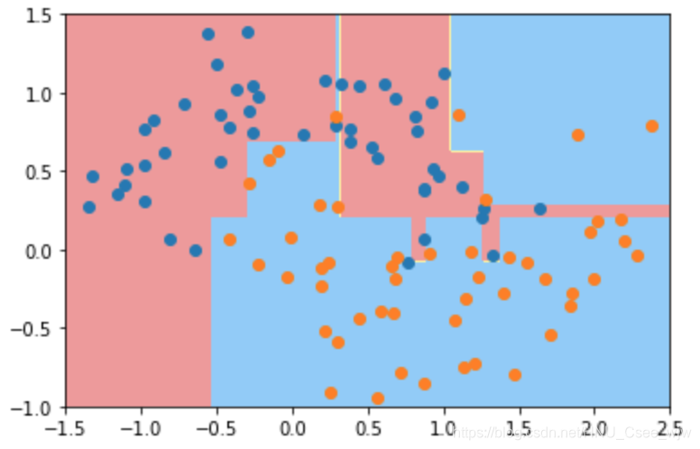

dt_clf2 = DecisionTreeClassifier(max_depth=2)
dt_clf2.fit(X, y)

plot_decision_boundary(dt_clf2, axis=[-1.5, 2.5, -1.0, 1.5])
plt.scatter(X[y==0,0], X[y==0,1])
plt.scatter(X[y==1,0], X[y==1,1])
plt.show()

dt_clf3 = DecisionTreeClassifier(min_samples_split=10) # 对于一个节点来说，只要有多少个样本数据才对其继续拆分
dt_clf3.fit(X, y)

plot_decision_boundary(dt_clf3, axis=[-1.5, 2.5, -1.0, 1.5])
plt.scatter(X[y==0,0], X[y==0,1])
plt.scatter(X[y==1,0], X[y==1,1])
plt.show()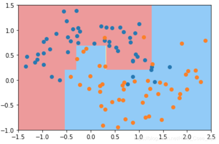

dt_clf4 = DecisionTreeClassifier(min_samples_leaf=6) # 对于一个叶子节点，最小应该有几个样本
dt_clf4.fit(X, y)

plot_decision_boundary(dt_clf4, axis=[-1.5, 2.5, -1.0, 1.5])
plt.scatter(X[y==0,0], X[y==0,1])
plt.scatter(X[y==1,0], X[y==1,1])
plt.show()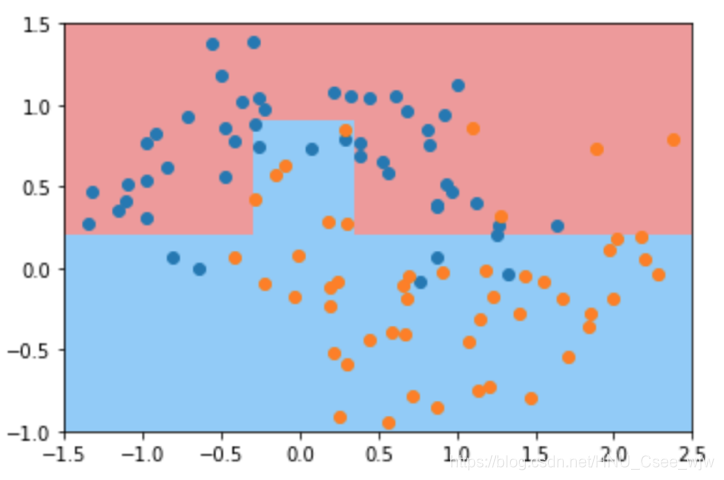

dt_clf5 = DecisionTreeClassifier(max_leaf_nodes=4) # 决策树最多有多少个叶子节点
dt_clf5.fit(X, y)

plot_decision_boundary(dt_clf5, axis=[-1.5, 2.5, -1.0, 1.5])
plt.scatter(X[y==0,0], X[y==0,1])
plt.scatter(X[y==1,0], X[y==1,1])
plt.show()

06 决策树解决回归问题

import numpy as np
import matplotlib.pyplot as plt

from sklearn import datasets

boston = datasets.load_boston()
X = boston.data
y = boston.target

from sklearn.model_selection import train_test_split

X_train, X_test, y_train, y_test = train_test_split(X, y, random_state=666)

Decision Tree Regressor

from sklearn.tree import DecisionTreeRegressor

dt_reg = DecisionTreeRegressor()
dt_reg.fit(X_train, y_train)
"""
Out[4]:
DecisionTreeRegressor(criterion='mse', max_depth=None, max_features=None,
           max_leaf_nodes=None, min_impurity_decrease=0.0,
           min_impurity_split=None, min_samples_leaf=1,
           min_samples_split=2, min_weight_fraction_leaf=0.0,
           presort=False, random_state=None, splitter='best')
"""

dt_reg.score(X_test, y_test)
# Out[5]:
# 0.58830200768338436

dt_reg.score(X_train, y_train) # 对训练集回归完全正确而测试集表现不好，说明过拟合
# Out[6]:
# 1.0

07 并查集的局限性

决策树的分类边界和理想的（斜线）有一定的差距

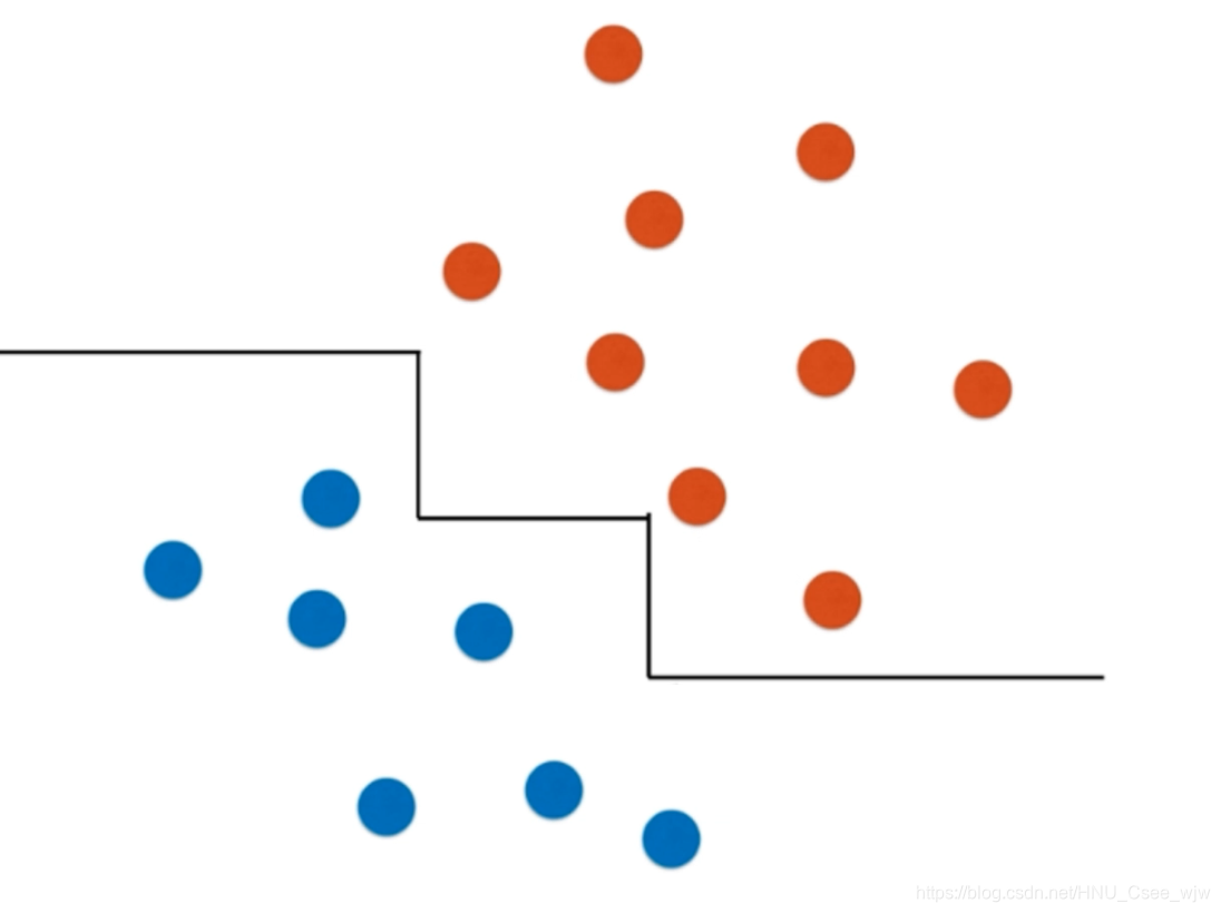
上图决策树绘制出的决策边界可能是错误的，尤其是在x，y接近无穷时的边界部分

缺点2：对个别样本点特别敏感，仿真如下：

import numpy as np
import matplotlib.pyplot as plt

from sklearn import datasets

iris = datasets.load_iris()
X = iris.data[:,2:]
y = iris.target

from sklearn.tree import DecisionTreeClassifier

tree_clf = DecisionTreeClassifier(max_depth=2, criterion='entropy')
tree_clf.fit(X, y)
"""
Out[3]:
DecisionTreeClassifier(class_weight=None, criterion='entropy', max_depth=2,
            max_features=None, max_leaf_nodes=None,
            min_impurity_decrease=0.0, min_impurity_split=None,
            min_samples_leaf=1, min_samples_split=2,
            min_weight_fraction_leaf=0.0, presort=False, random_state=None,
            splitter='best')
"""
def plot_decision_boundary(model, axis):
    
    x0, x1 = np.meshgrid(
        np.linspace(axis[0], axis[1], int((axis[1]-axis[0])*100)).reshape(-1,1),
        np.linspace(axis[2], axis[3], int((axis[3]-axis[2])*100)).reshape(-1,1)
    )
    X_new = np.c_[x0.ravel(), x1.ravel()]
    
    y_predict = model.predict(X_new)
    zz = y_predict.reshape(x0.shape)
    
    from matplotlib.colors import ListedColormap
    custom_cmap = ListedColormap(['#EF9A9A', '#FFF59D','#90CAF9'])
    
    plt.contourf(x0, x1, zz, linewidth=5, cmap=custom_cmap)

plot_decision_boundary(tree_clf, axis=[0.5, 7.5, 0, 3])
plt.scatter(X[y==0,0], X[y==0,1])
plt.scatter(X[y==1,0], X[y==1,1])
plt.scatter(X[y==2,0], X[y==2,1])
plt.show()

# 删除第138行数据
X_new = np.delete(X, 137, axis=0)
y_new = np.delete(y, 137)

X_new.shape
# Out[7]:
# (149, 2)

y_new.shape
# Out[8]:
# (149,)

tree_clf2 = DecisionTreeClassifier(max_depth=2, criterion='entropy')
tree_clf2.fit(X_new, y_new)
"""
Out[9]:
DecisionTreeClassifier(class_weight=None, criterion='entropy', max_depth=2,
            max_features=None, max_leaf_nodes=None,
            min_impurity_decrease=0.0, min_impurity_split=None,
            min_samples_leaf=1, min_samples_split=2,
            min_weight_fraction_leaf=0.0, presort=False, random_state=None,
            splitter='best')
"""
plot_decision_boundary(tree_clf2, axis=[0.5, 7.5, 0, 3])
plt.scatter(X[y==0,0], X[y==0,1])
plt.scatter(X[y==1,0], X[y==1,1])
plt.scatter(X[y==2,0], X[y==2,1])
plt.show()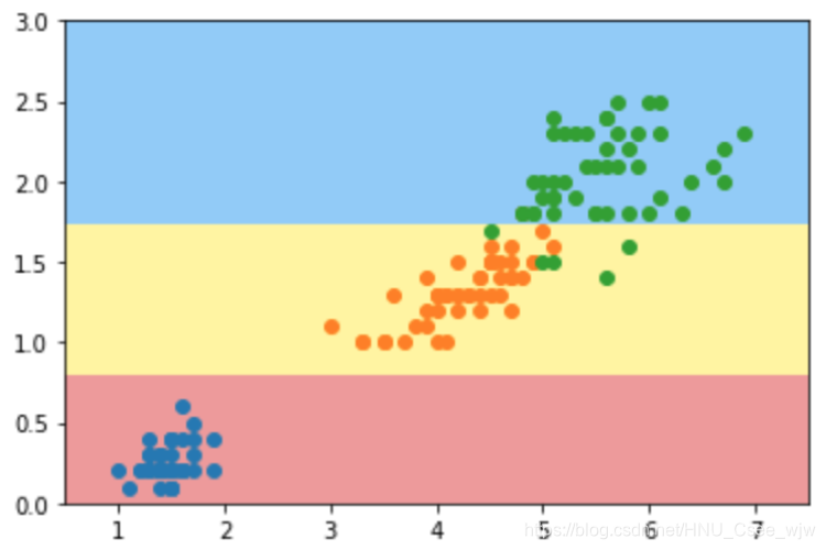

最后，如果有什么疑问，欢迎和我微信交流。

Python遇见机器学习 ---- 决策树 Decision Tree

综述