文本分布式表示（二）：用tensorflow和word2vec训练词向量

看了几天word2vec的理论，终于是懂了一些。理论部分我推荐以下几篇教程，有博客也有视频：

1、《word2vec中的数学原理》：http://www.cnblogs.com/peghoty/p/3857839.html
2、刘建平：word2vec原理：https://www.cnblogs.com/pinard/p/7160330.html
3、吴恩达：《序列模型：自然语言处理与词嵌入》

理论看完了就要实战了，通过实战能加深对word2vec的理解。目前用word2vec算法训练词向量的工具主要有两种：gensim 和 tensorflow。gensim中已经封装好了word2vec这个包，用起来很方便，只要把文本处理成规范的输入格式，寥寥几行代码就能训练词向量。这样比较适合在做项目时提高效率，但是对理解算法的原理帮助不大。相比之下，用tensorflow来训练word2vec比较麻烦，生成batch、定义神经网络的各种参数，都要自己做，但是对于理解算法原理，还是帮助很大。

所以这次就用开源的tensorflow实现word2vec的代码，来训练词向量，并进行可视化。这次的语料来自于一个新闻文本分类的项目，没学word2vec之前已经做了那个项目，但是对embedding那一部分不清楚。现在打算把词向量训练好后，看怎么在文本分类项目中用起来。当然这是以后的任务，这次的任务就是训练词向量和可视化。

这篇博客的主体分为两部分，第一部分是展示怎样用微调的tensorflow开源代码来训练自己的语料，会对代码进行比较详细地解读和注解；第二部分是我在解读代码的过程中，整理的python和tensorflow语法知识，基本上难一点的代码都有解释和案例，我觉得对刚接触的人会比较有好处。

新闻文本文档非常大，有 120多M，这里提供百度网盘下载：https://pan.baidu.com/s/1yeFORUVr3uDdTLUYqDraKA 提取码：c98y

词向量训练出来有715M，真是醉了！好，开始吧。

一、用tensorflow和word2vec训练中文词向量

这次用到的是skip-gram模型。新闻文本的训练语料是一个txt文档，每行是一篇新闻，开头两个字是标签：体育、财经、娱乐等，后面是新闻的内容，开头和内容之间用制表符 '\t' 隔开。

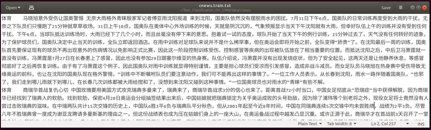
（一）读取文本数据，分词，清洗，生成符合输入格式的内容

这里是用jieba进行分词的，加载了停用词表，不加载的话会发现 “的、一 ”之类的词是排在前列的，而负采样是从词频高的词开始，因此会对结果产生不好的影响。

处理得到的规范格式的输入是这样的，把所有新闻文本分词后做成一个列表：['体育', '马', '晓', '旭', '意外', '受伤', '国奥', '警惕', '无奈', '大雨', ...]。

#encoding=utf8
from __future__ import absolute_import
from __future__ import division
from __future__ import print_function

import collections
import math
import os
import random
import zipfile

import numpy as np
from six.moves import xrange  
import tensorflow as tf
import jieba
from itertools import chain

# 第一步：读取数据，用jieba进行分词，去除停用词，生成词语列表。

def read_data(filename):
    f = open(filename, 'r',  encoding='utf-8')
    stop_list = [i.strip() for i in open('ChineseStopWords.txt','r',encoding='utf-8')]          # 读取停用词表
    news_list = []
    for line in f:                # line是：'体育\t马晓旭意外受伤让国奥警惕 无奈大雨格外...'这样的新闻文本，标签是‘体育’，后面是正文，中间用'\t'分开。
        if line.strip():
            news_cut = list(jieba.cut(''.join(line.strip().split('\t')),cut_all=False,HMM=False))  
            # ['体育', '马', '晓', '旭', '意外', '受伤', '让', '国奥', '警惕', ' ', '无奈',...], 按'\t'来拆开
            news_list.append([word.strip() for word in news_cut if word not in stop_list and len( word.strip())>0]) 
            #news_list为[['体育', '马', '晓', '旭', '意外', '受伤', '国奥', '警惕', '无奈', ...]，去掉了停用词和空格。

    news_list = list(chain.from_iterable(news_list))             # 原列表中的元素也是列表，把它拉成一个列表。['体育', '马', '晓', '旭', '意外', '受伤', '国奥', '警惕', '无奈', '大雨', ...]
    f.close()
    return news_list

filename = 'data/cnews/cnews.train.txt'
words = read_data(filename)                 # 把所有新闻分词后做成了一个列表：['体育', '马', '晓', '旭', '意外', '受伤', '国奥', '警惕', '无奈', '大雨', ...]

（二）建立词汇表

这一步是把得到的词列表中的词去重，统计词频，然后按词频从高到低排序，构建一个词汇表：{'UNK': 0, '中': 1, '月': 2, '年': 3, '说': 4, '中国': 5,...}，key是词，‘中’的词频最高，放在前面，value是每个词的索引。

为了便于根据索引来取词，因此把词汇表这个字典进行反转得到：reverse_dictionary: {0: 'UNK', 1: '中', 2: '月', 3: '年', 4: '说', 5: '中国',...}。

同时还得到了上面words这个列表中每个词的索引： [259, 512, 1023, 3977, 1710, 1413, 12286, 6118, 2417, 18951, ...]。

词语（含重复）共有1545万多个，去重复后得到19万多个。

# 第二步：建立词汇表

words_size = len(words)      # 共有15457860个，重复的词非常多。
vocabulary_size = len(set(words))      # 词汇表中有196871个不同的词。
print('Data size', vocabulary_size)     

def build_dataset(words):
    count = [['UNK', -1]]
    count.extend(collections.Counter(words).most_common(vocabulary_size - 1))    #统计词频较高的词，并得到词的词频。
    # count[:10]: [['UNK', -1], ('中', 96904), ('月', 75567), ('年', 73174), ('说', 56859), ('中国', 55539), ('日', 54018), ('%', 52982), ('基金', 47979), ('更', 40396)]
    #  尽管取了词汇表前（196871-1）个词，但是前面加上了一个用来统计未知词的元素，所以还是196871个词。之所以第一个元素是列表，是为了便于后面统计未知词的个数。
    dictionary = dict()
    for word, _ in count:
        dictionary[word] = len(dictionary)
    # dictionary: {'UNK': 0, '中': 1, '月': 2, '年': 3, '说': 4, '中国': 5,...}，是词汇表中每个字是按照词频进行排序后，字和它的索引构成的字典。
    data = list()
    unk_count = 0
    for word in words:
        if word in dictionary:
            index = dictionary[word]
        else:
            index = 0  # dictionary['UNK']
            unk_count += 1
        data.append(index)
        # data是words这个文本列表中每个词对应的索引。元素和words一样多，是15457860个
        # data[:10] : [259, 512, 1023, 3977, 1710, 1413, 12286, 6118, 2417, 18951]
    
    count[0][1] = unk_count       # 位置词就是'UNK'本身，所以unk_count是1。[['UNK', 1], ('中', 96904), ('月', 75567), ('年', 73174), ('说', 56859), ('中国', 55539),...]
    reverse_dictionary = dict(zip(dictionary.values(), dictionary.keys()))       # 把字典反转：{0: 'UNK', 1: '中', 2: '月', 3: '年', 4: '说', 5: '中国',...}，用于根据索引取词。
    return data, count, dictionary, reverse_dictionary

data, count, dictionary, reverse_dictionary = build_dataset(words)
# data[:5] : [259, 512, 1023, 3977, 1710]
# count[:5]: [['UNK', 1], ('中', 96904), ('月', 75567), ('年', 73174), ('说', 56859)]
# reverse_dictionary: {0: 'UNK', 1: '中', 2: '月', 3: '年', 4: '说', 5: '中国',...}

del words          # 删掉不同的数据，释放内存。
print('Most common words (+UNK)', count[:5])
print('Sample data', data[:10], [reverse_dictionary[i] for i in data[:10]])

# Most common words (+UNK) [['UNK', 1], ('中', 96904), ('月', 75567), ('年', 73174), ('说', 56859)]
# Sample data [259, 512, 1023, 3977, 1710, 1413, 12286, 6118, 2417, 18951] ['体育', '马', '晓', '旭', '意外', '受伤', '国奥', '警惕', '无奈', '大雨']

（三）为skip-gram模型生成训练的batch

skip-gram模型是根据中心词来预测上下文词的，拿['体育', '马', '晓', '旭', '意外', '受伤', '国奥', '警惕', '无奈', '大雨']来举例，滑动窗口为5，那么中心词前后各2个词，第一个中心词为 ‘晓’时，上下文词为(体育，马，旭，意外)这样一个没有顺序的词袋。

那么生成的样本可能为：[（晓，马），（晓，意外），（晓，体育），（晓，旭）]，上下文词不是按顺序排列的。

# 第三步：为skip-gram模型生成训练的batch

def generate_batch(batch_size, num_skips, skip_window):
    global data_index
    assert batch_size % num_skips == 0
    assert num_skips <= 2 * skip_window
    batch = np.ndarray(shape=(batch_size), dtype=np.int32)          # 这里先取一个数量为8的batch看看，真正训练时是以128为一个batch的。
    labels = np.ndarray(shape=(batch_size, 1), dtype=np.int32)     #  构造一个一列有8个元素的ndarray对象
    span = 2 * skip_window + 1  # [ skip_window target skip_window ]
    buffer = collections.deque(maxlen=span)      # deque 是一个双向列表,限制最大长度为5， 可以从两端append和pop数据。
    for _ in range(span): 
        buffer.append(data[data_index])
        data_index = (data_index + 1) % len(data)      
        # 循环结束后得到buffer为 deque([259, 512, 1023, 3977, 1710], maxlen=5)，也就是取到了data的前五个值, 对应词语列表的前5个词。
    
    for i in range(batch_size // num_skips):      #i取值0,1，是表示一个batch能取两个中心词
        target = skip_window         # 值为2，意思是中心词在buffer这个列表中的位置是2。
        targets_to_avoid = [skip_window]       # 这个列表是用来存已经取过的词的索引，下次就不能再取了，从而把buffer中5个元素不重复地取完。
        for j in range(num_skips):        #j取0，1，2，3，意思是在中心词周围取4个词。
            while target in targets_to_avoid:
                target = random.randint(0, span - 1)      # 2是中心词的位置，所以j的第一次循环要取到不是2的数字，也就是取到0，1，3，4其中的一个，才能跳出循环。
            targets_to_avoid.append(target)                 # 把取过的上下文词的索引加进去。
            batch[i * num_skips + j] = buffer[skip_window]         # 取到中心词的索引。前四个元素都是同一个中心词的索引。
            labels[i * num_skips + j, 0] = buffer[target]              # 取到中心词的上下文词的索引。一共会取到上下各两个。
        buffer.append(data[data_index])             
        # 第一次循环结果为buffer：deque([512, 1023, 3977, 1710, 1413], maxlen=5)，所以明白了为什么限制为5，因为可以把第一个元素去掉。这也是为什么不用list。
        data_index = (data_index + 1) % len(data)
    return batch, labels

batch, labels = generate_batch(batch_size=8, num_skips=4, skip_window=2)
# batch是 array([1023, 1023, 1023, 1023, 3977, 3977, 3977, 3977], dtype=int32)，8个batch取到了2个中心词，一会看样本的输出结果就明白了。
for i in range(8):
    print(batch[i], reverse_dictionary[batch[i]],
        '->', labels[i, 0], reverse_dictionary[labels[i, 0]])
'''
打印的结果如下，突然明白说为什么说取样本的时候是用bag of words

1023 晓 -> 3977 旭
1023 晓 -> 1710 意外
1023 晓 -> 512 马
1023 晓 -> 259 体育
3977 旭 -> 512 马
3977 旭 -> 1023 晓
3977 旭 -> 1710 意外
3977 旭 -> 1413 受伤
'''

（四）定义skip-gram模型

这里面涉及的一些tensorflow的知识点在第二部分有写，这里也说明一下。

首先 tf.Graph().as_default() 表示将新生成的图作为整个 tensorflow 运行环境的默认图，如果只有一个主线程不写也没有关系，tensorflow 里面已经存好了一张默认图，可以使用tf.get_default_graph() 来调用（显示这张默认纸），当你有多个线程就可以创造多个tf.Graph()，就是你可以有一个画图本，有很多张图纸，而默认的只有一张，可以自己指定。

tf.random_uniform这个方法是用来产生-1到1之间的均匀分布, 看作是初始化隐含层和输出层之间的词向量矩阵。

nce_loss函数是tensorflow中常用的损失函数，可以将其理解为其将多元分类分类问题强制转化为了二元分类问题，num_sampled参数代表将选取负例的个数。

这个损失函数通过 sigmoid cross entropy来计算output和label的loss，从而进行反向传播。这个函数把最后的问题转化为了（num_sampled ，num_True）这个两分类问题，然后每个分类问题用了交叉熵损失函数。

# 第四步：定义skip-gram模型的参数、损失函数

# 首先定义参数
batch_size = 128            # 上面那个数量为8的batch只是为了展示以下取样的结果，实际上是batch-size 是128。
embedding_size = 300   # 词向量的维度是300维。
skip_window = 2             # 左右两边各取两个词。
num_skips = 4                # 要取4个上下文词，同一个中心词也要重复取4次。
num_sampled = 64        # 负采样的负样本数量为64

graph = tf.Graph()         # 新生成一张计算图

with graph.as_default():                   #  把新生成的图作为整个 tensorflow 运行环境的默认图，详见第二部分的知识点。

    train_inputs = tf.placeholder(tf.int32, shape=[batch_size])        
    train_labels = tf.placeholder(tf.int32, shape=[batch_size, 1])      #placeholder()函数是在神经网络构建graph的时候在模型中的占位，它只会分配必要的内存

    embeddings = tf.Variable(tf.random_uniform([vocabulary_size, embedding_size], -1.0, 1.0))
   # 产生-1到1之间的均匀分布, 看作是初始化隐含层和输出层之间的词向量矩阵。
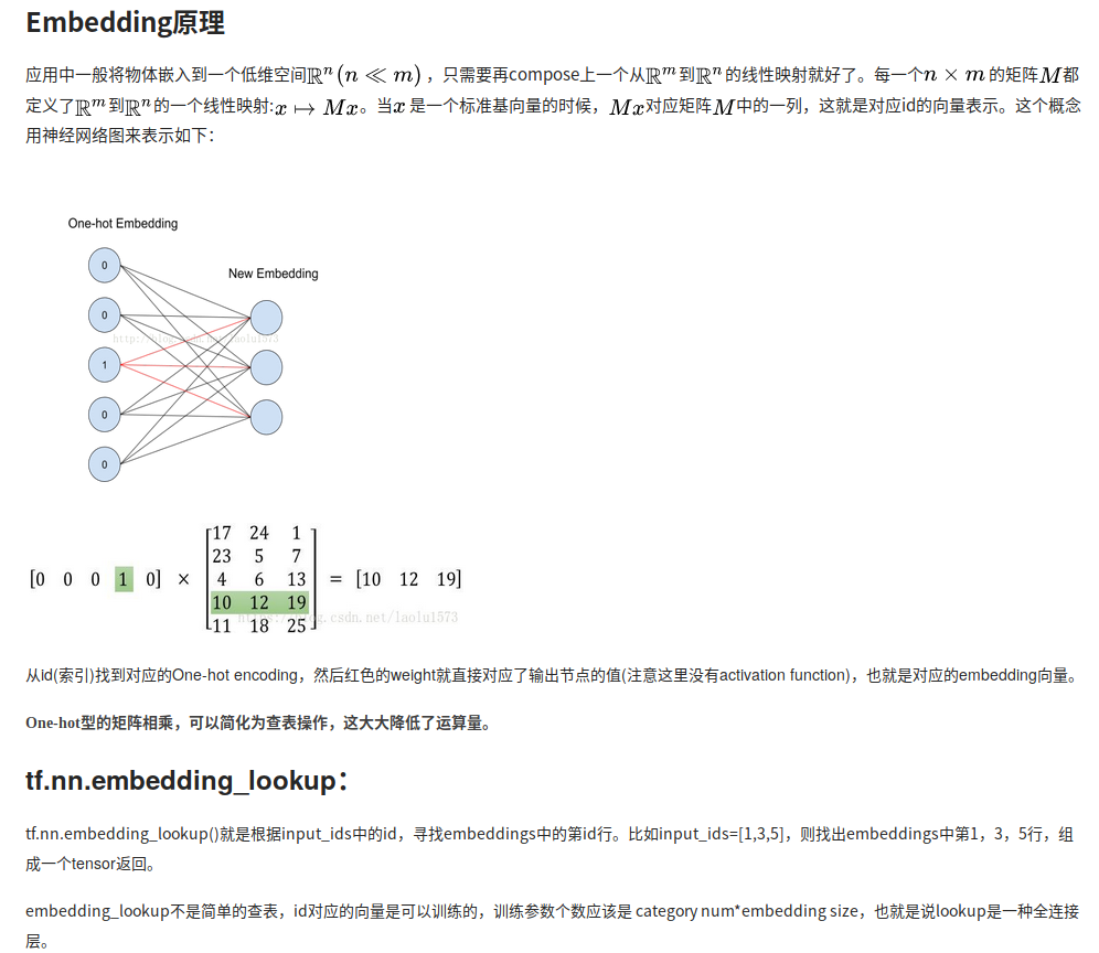
    embed = tf.nn.embedding_lookup(embeddings, train_inputs)             #用词的索引在词向量矩阵中得到对应的词向量。shape=(128, 300)

    # 初始化损失（loss）函数的权重矩阵和偏置矩阵
    nce_weights = tf.Variable(tf.truncated_normal([vocabulary_size, embedding_size], stddev=1.0 / math.sqrt(embedding_size)))
    # 生成的值服从具有指定平均值和合理标准偏差的正态分布，如果生成的值大于平均值2个标准偏差则丢弃重新生成。这里是初始化权重矩阵。
    # 对标准方差进行了限制的原因是为了防止神经网络的参数过大。

    nce_biases = tf.Variable(tf.zeros([vocabulary_size])) #初始化偏置矩阵，生成了一个vocabulary_size * 1大小的零矩阵。

    loss = tf.reduce_mean(tf.nn.nce_loss(weights=nce_weights, biases=nce_biases,
                 labels=train_labels, inputs=embed, num_sampled=num_sampled, num_classes=vocabulary_size))
    # 这个tf.nn.nce_loss函数把多分类问题变成了正样本和负样本的二分类问题。用的是逻辑回归的交叉熵损失函数来求，而不是softmax  。

    # 用的是SGD梯度下降法，每次只传入一个样本去计算，学习率为1
    optimizer = tf.train.GradientDescentOptimizer(1.0).minimize(loss)

    norm = tf.sqrt(tf.reduce_sum(tf.square(embeddings), 1, keepdims=True))       # shape=(196871, 1), 和下面的代码一起，对词向量矩阵进行归一化。
    normalized_embeddings = embeddings / norm


    init = tf.global_variables_initializer()          # 初始化所有的变量。

（五）训练skip-gram模型

接下来就开始训练了，这里没什么好说的，就是训练神经网络，不断更新词向量矩阵，然后训练完后，得到最终的词向量矩阵。源码中还有一个展示邻近词语的代码，我觉得没啥用，删掉了。

num_steps = 10     # 训练10轮，每轮128个batch。
with tf.Session(graph=graph) as session:

    init.run()
    print('initialized.')
    average_loss = 0

    for step in xrange(num_steps):
        # 产生一个minibatch 
        batch_inputs, batch_labels = generate_batch(batch_size, num_skips, skip_window)
        feed_dict = {train_inputs: batch_inputs, train_labels: batch_labels}
   
        _, loss_val = session.run([optimizer, loss], feed_dict=feed_dict)
        average_loss += loss_val
        final_embeddings = normalized_embeddings.eval()
        print(final_embeddings)        
        print("*"*20)
      
        if step % 2000 == 0:
            if step > 0:
                average_loss /= 2000
            print("Average loss at step ", step, ": ", average_loss)
            average_loss = 0
        
    final_embeddings = normalized_embeddings.eval()      # 训练得到最后的词向量矩阵。说实话我也不太懂怎么就得到了。
    print(final_embeddings)
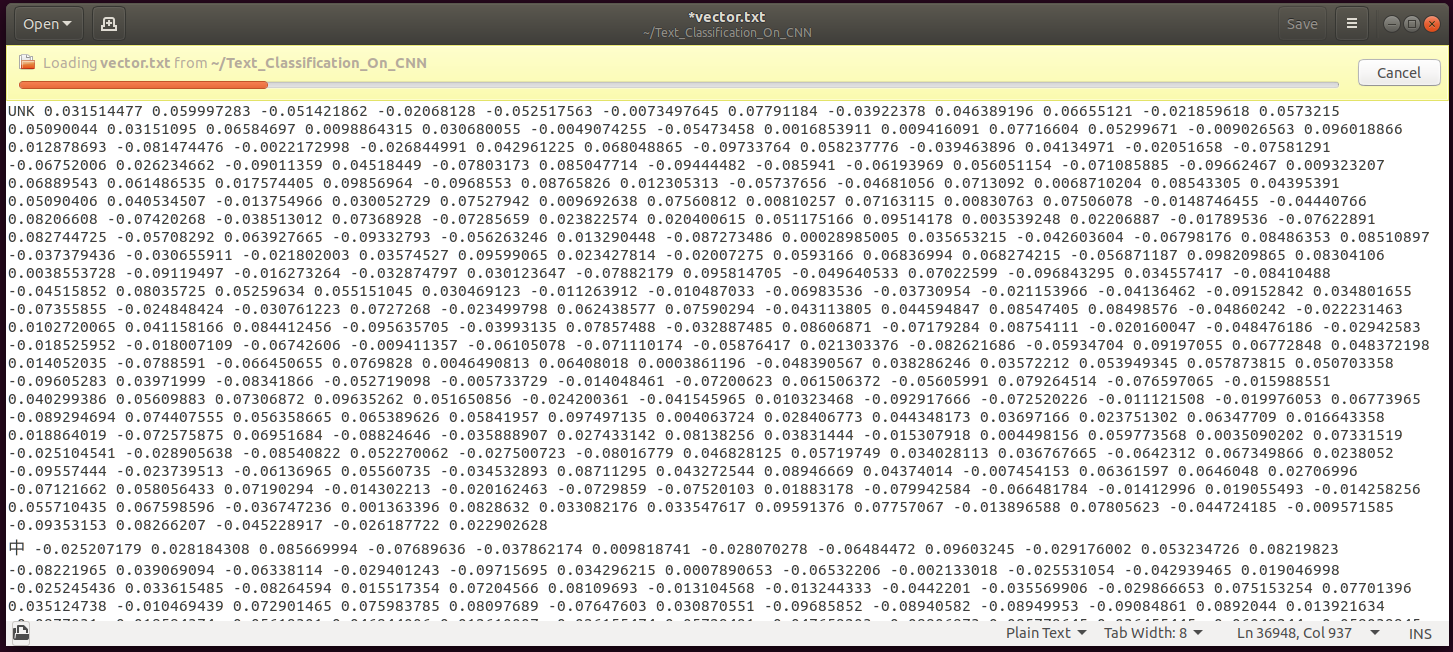
    fp=open('vector.txt','w',encoding='utf8')
    for k,v in reverse_dictionary.items():
        t=tuple(final_embeddings[k])         # (0.031514477, 0.059997283, -0.051421862, -0.02068128, ...)  取出词汇表中每一个词的词向量。
        s=''
        for i in t:
            i=str(i)
            s+=i+" "               #s为'0.031514477 0.059997283 ...'  , 对于每一个词的词向量中的300个数字，用空格把他们连接成字符串。
        fp.write(v+" "+s+"\n")         #把词向量写入文本文档中。不过这样就成了字符串，我之前试过用np保存为ndarray格式，这里是按源码的保存方式。
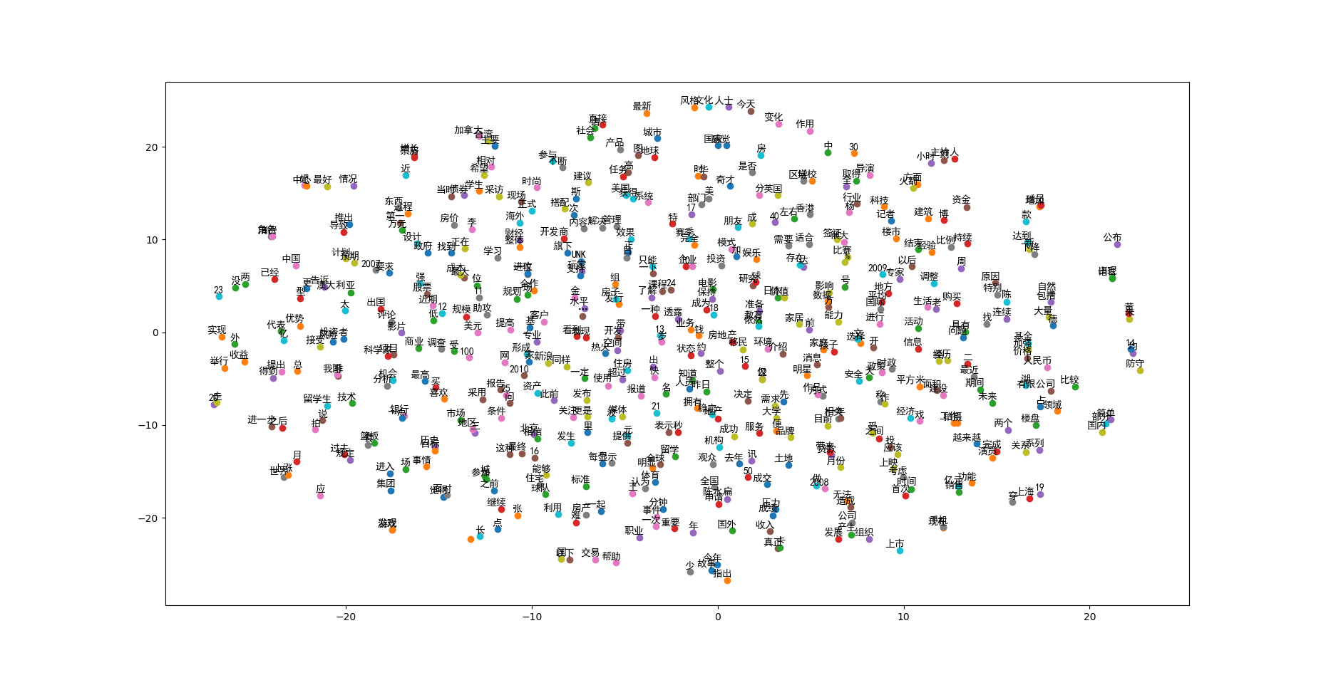
    fp.close()

（六）词向量可视化

用sklearn.manifold.TSNE这个方法来进行可视化，实际上作用不是画图，而是降维，因为词向量是300维的，降到2维或3维才能可视化。

这里用到了t-SNE这一种集降维与可视化于一体的技术，t-SNE 的主要目的是高维数据的可视化，当数据嵌入二维或三维时，效果最好。

值得注意的一点是，matplotlib默认的字体是不含中文的，所以没法显示中文注释，要自己导入中文字体。在默认状态下，matplotlb无法在图表中使用中文。

matplotlib中有一个字体管理器——matplotlib.Font_manager,通过该管理器的方法——matplotlib.Font_manager.FontProperties(fname)可以指定一个ttf字体文件作为图表使用的字体。

# 第六步：词向量可视化。
def plot_with_labels(low_dim_embs, labels, filename='tsne.png'):
    assert low_dim_embs.shape[0] >= len(labels), "More labels than embeddings"
    plt.figure(figsize=(18, 18))  # in inches
    myfont = font_manager.FontProperties(fname='/home/dyy/Downloads/font163/simhei.ttf')   #加载中文字体
    for i, label in enumerate(labels):
        x, y = low_dim_embs[i, :]
        plt.scatter(x, y)
        plt.annotate(label,
                 xy=(x, y),
                 xytext=(5, 2),                           #添加注释, xytest是注释的位置。然后添加显示的字体。
                 textcoords='offset points',
                 ha='right',
                 va='bottom',
                 fontproperties=myfont)

    plt.savefig(filename)
    plt.show()

try:
    from sklearn.manifold import TSNE
    import matplotlib.pyplot as plt
    from matplotlib import font_manager            #这个库很重要，因为需要加载字体，原开源代码里是没有的。

    tsne = TSNE(perplexity=30, n_components=2, init='pca', n_iter=5000)         # 一个降维的方法，降维后维度是2维，使用'pca'来初始化。
    plot_only = 500
    low_dim_embs = tsne.fit_transform(final_embeddings[:plot_only, :])           #取出了前500个词的词向量，把300维减低到2维。
    labels = [reverse_dictionary[i] for i in xrange(plot_only)]            # 把这500个词取出来。
    plot_with_labels(low_dim_embs, labels)

except ImportError:
    print("Please install sklearn, matplotlib, and scipy to visualize embeddings.")

可视化的结果：

词向量（太大了，打开也要花不少时间）

二、相关知识点整理

1 python知识：zipfile 解压文件

解压：

1 f=zipfile.ZipFile(file, mode="r")：解压一个zip文件对象。

2 ZipFile.namelist() ：返回文件列表

3 ZipFile.read(name[, mode[, password]]) ：打开压缩文档中的某个文件

压缩

1、f=zipfile.ZipFile(file, mode="w"): 如果是压缩则需要把mode改为‘w’，并创建一个zip文件。

2、f.write(filename)：将文件写入zip文件中，即将文件压缩

f.close（）

将zip文件对象关闭，与open一样可以使用上下文with...as f。

import zipfile

with zipfile.ZipFile('text8.zip') as f:
    print(f.namelist())
    print(f.read(f.namelist()[0]))  # 数据量太大了，无法读取，但是语法是对的。

['test_seg.txt']

IOPub data rate exceeded.
The notebook server will temporarily stop sending output
to the client in order to avoid crashing it.
To change this limit, set the config variable
`--NotebookApp.iopub_data_rate_limit`.

Current values:
NotebookApp.iopub_data_rate_limit=1000000.0 (bytes/sec)
NotebookApp.rate_limit_window=3.0 (secs)

2 python知识：collections.Counter()

使用collections.Counter类统计列表元素出现次数

from collections import Counter

names = ["Stanley", "Lily", "Bob", "Well", "Peter", "Bob", "Well", "Peter", "Well", "Peter", "Bob",\
      "Stanley", "Lily", "Bob", "Well", "Peter", "Bob", "Bob", "Well", "Peter", "Bob", "Well"]
print(Counter(names))  # 得到一个字典，可以根据名字得到它的频率
print(Counter(names).most_common(3))  # 得到频率最高的前几个词及其频率的元祖，构成一个列表

Counter({'Bob': 7, 'Well': 6, 'Peter': 5, 'Stanley': 2, 'Lily': 2})
[('Bob', 7), ('Well', 6), ('Peter', 5)]

3 python知识：assert函数

参考资料

1 一般的用法是：assert condition

2 用来让程序测试这个condition，如果condition为false，那么raise一个AssertionError出来。逻辑上等同于：

if not condition:
    raise AssertionError()
    

3 assert断言语句添加异常参数: 其实就是在断言表达式后添加字符串信息，用来解释断言并更好的知道是哪里出了问题。

格式如下：

assert expression [, arguments]

# 条件为真时
assert 1==1

# 条件为假时
assert 1==0

---------------------------------------------------------------------------

AssertionError                            Traceback (most recent call last)

<ipython-input-10-78e0964adc84> in <module>
      1 # 条件为假时
----> 2 assert 1==0

AssertionError: 

# 添加异常参数
assert 2==1,'2不等于1'

---------------------------------------------------------------------------

AssertionError                            Traceback (most recent call last)

<ipython-input-11-3bb55e7263f1> in <module>
      1 # 添加异常参数
----> 2 assert 2==1,'2不等于1'

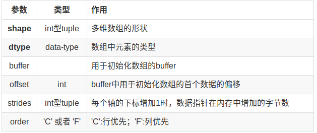
AssertionError: 2不等于1

4 python知识：np.ndarray()

numpy.ndarray()是numpy的构造函数，我们可以使用这个函数创建一个ndarray对象.

# 随机生成ndarray对象，不传入原始数组
import numpy as np

np.ndarray(shape=(2,3),dtype=int)

array([[4121128125901447780, 3554525595036758061, 3329060874566515252],
       [2475346127859823155, 7236833184642769452, 7881144752318672485]])

# 把已有的数组构造成ndarray对象,按照行优先，数组中的数据超过时，把靠后的多余的数据去掉。
import numpy as np

np.ndarray(shape=(2,3), dtype=int, buffer=np.array([1,2,3,4,5,6,7]), offset=0, order="C")

array([[1, 2, 3],
       [4, 5, 6]])

# 把已有的数组构造成ndarray对象,按照列优先，数组中的数据超过时，把靠前的多余的数据去掉。
import numpy as np

np.ndarray(shape=(2,3), dtype=int, buffer=np.array([1,2,3,4,5,6,7]), offset=8, order="F")

array([[2, 4, 6],
       [3, 5, 7]])

5 python知识：collections.deque

1 deque是为了高效实现插入和删除操作的双向列表，适合用于队列和栈。deque结构可以看作是内置的list结构的加强版,且比队列提供了更强大的方法.

2 deque 是 double-ended queue的缩写，类似于 list，不过提供了在两端插入和删除的操作。

appendleft: 在列表左侧插入
popleft: 弹出列表左侧的值

from collections import deque

q = deque(['a', 'b', 'c'])  # 把list的各项添加到双向列表中
q.append('x') # 这个和一般的list一样，在末尾添加
q.appendleft('y')  # 这个是独有的功能，在开头添加
print(q)

deque(['y', 'a', 'b', 'c', 'x'])

# 限制deque的长度
from collections import deque

d = deque(maxlen=5)
for i in range(10):
    d.append(str(i))

print(d)

#可见当限制长度的deque增加超过限制数的项时，另一边的项会自动删除。

deque(['5', '6', '7', '8', '9'], maxlen=5)

6 python知识：np.random.choice()

用途：

可以从一个int数字或1维array里随机选取内容，并将选取结果放入n维array中返回。

说明：

numpy.random.choice(a, size=None, replace=True, p=None)

参数意思分别是从a中按照每个元素被抽到的概率P，随机选择size个, p没有指定的时候相当于是一致的分布。

replacement 代表的意思是抽样之后还放不放回去，如果是False的话，那么出来的三个数都不一样，如果是

True的话， 有可能会出现重复的，因为前面的抽的放回去了。

import numpy as np

valid_size = 16 
valid_window = 100 
# 从range（100）中抽取16个不重复的数字。False表示不重复
valid_examples = np.random.choice(valid_window, valid_size, replace=False) # 第一个参数可以使一个数字，也可以是列表。
print(valid_examples)

[ 1 67 12 28 48 40 84 71 20 24 34 90 29 73 58  4]

import numpy as np

arr = ['pooh', 'rabbit', 'piglet', 'Christopher']
np.random.choice(arr, 5, p=[0.5, 0.1, 0.1, 0.3]) # ‘pooh’的概率为0.5，最大，所以被抽到的概率最大，抽到两次。

array(['rabbit', 'pooh', 'Christopher', 'Christopher', 'pooh'],
      dtype='<U11')

7 tensorflow知识：graph.as_default()和tf.Graph()

【1】 tf.Graph() 表示实例化了一个类，一个用于 tensorflow 计算和表示用的数据流图，通俗来讲就是：在代码中添加的操作（画中的结点）和数据（画中的线条）都是画在纸上的“画”，而图就是呈现这些画的纸，你可以利用很多线程生成很多张图，但是默认图就只有一张。

【2】 tf.Graph().as_default() 表示将这个类实例，也就是新生成的图作为整个 tensorflow 运行环境的默认图，如果只有一个主线程不写也没有关系，tensorflow 里面已经存好了一张默认图，可以使用tf.get_default_graph() 来调用（显示这张默认纸），当你有多个线程就可以创造多个tf.Graph()，就是你可以有一个画图本，有很多张图纸，而默认的只有一张，可以自己指定。

import tensorflow as tf

c = tf.constant(4.0)
assert c.graph is tf.get_default_graph() # c是在默认的图里面

g = tf.Graph()  # 新建了一张图，并把它设为默认图，于是就有了两张图。
with g.as_default():
    c = tf.constant(30.0)  # 这个常量是在新图里面。
    assert c.graph is g

'''
最终结果是没有报错
'''

'\n最终结果是没有报错\n'

8 tensorflow知识：tf.placeholder

【1】含义

Tensorflow的设计理念称之为计算流图，在编写程序时，首先构筑整个系统的graph，代码并不会直接生效，这一点和python的其他数值计算库（如Numpy等）不同，graph为静态的，类似于docker中的镜像。然后，在实际的运行时，启动一个session，程序才会真正的运行。

所以placeholder()函数是在神经网络构建graph的时候在模型中的占位，此时并没有把要输入的数据传入模型，它只会分配必要的内存。等建立session，在会话中，运行模型的时候通过feed_dict()函数向占位符喂入数据。

【2】语法

tf.placeholder(
    dtype,
    shape=None,
    name=None
)

参数：

dtype：数据类型。常用的是tf.float32,tf.float64等数值类型
shape：数据形状。默认是None，就是一维值，也可以是多维（比如[2,3], [None, 3]表示列是3，行不定）
name：名称

import tensorflow as tf
import numpy as np

x = tf.placeholder(tf.float32, shape=(1024, 1024))
y = tf.matmul(x,x) # 定义好静态的计算

with tf.Session() as sess:
    rand_array = np.random.rand(1024,1024)
    print(sess.run(y,feed_dict={x:rand_array}))  # 传入数据，sess.run的时候才是真正开始运行程序的时候。

[[256.96985 257.1845  257.91666 ... 253.41881 261.50443 255.10269]
 [250.55695 250.10742 252.77834 ... 247.17044 255.52808 253.16248]
 [254.66516 258.60193 258.69525 ... 258.425   265.1694  254.95067]
 ...
 [266.63342 263.67966 269.86865 ... 265.58093 270.3124  262.35416]
 [252.40651 243.87204 253.63457 ... 248.87032 254.61702 252.23233]
 [253.44269 250.27487 252.86223 ... 253.26025 258.06012 250.55937]]

9 tensorflow知识：tf.random_uniform

tf.random_uniform((4, 4), minval=low,maxval=high,dtype=tf.float32)))返回4*4的矩阵，值位于low和high之间，服从均匀分布

import tensorflow as tf
import numpy as np

var = tf.random_uniform([4,4],minval=-1,maxval=1,dtype=tf.float32)

with tf.Session() as sess: 
    print(sess.run(var))

[[-0.7687669  -0.5589919   0.44953084 -0.71320367]
 [ 0.45806217  0.31792617 -0.85152483  0.91512346]
 [ 0.18106127 -0.8571527   0.7447574  -0.45698404]
 [ 0.8409984  -0.2989726   0.20090222 -0.96967053]]

10 tensorflow知识: tf.nn.embedding_lookup()

参考资料

# coding=utf-8
import tensorflow as tf 
import numpy as np # 定义一个未知变量input_ids用于存储索引

input_ids = tf.placeholder(dtype=tf.int32, shape=[5]) # 输入的词有5个。
embedding = tf.Variable(tf.random_uniform([20, 10], -1.0, 1.0)) # 词向量矩阵是20*10的，表示20个词，嵌入维度是10。

input_embedding = tf.nn.embedding_lookup(embedding, input_ids) # 找到5个词对应的词向量

with tf.Session() as sess:
    sess.run(tf.global_variables_initializer()) 
    print(sess.run(input_embedding, feed_dict={input_ids: [3,6,9,11,2]})) # 根据词的id来找，注意是这是一个行向量。

[[-0.40510893 -0.9786329  -0.18972254  0.80751324  0.14117026 -0.7359052
  -0.3441372  -0.7869594   0.08810854 -0.38642383]
 [ 0.44669318 -0.68000245  0.5797839  -0.19882703 -0.40526843  0.33085847
  -0.59173083  0.78422284 -0.12500834 -0.3774383 ]
 [ 0.01742125  0.14982057  0.15930486 -0.5717144   0.8315854  -0.8036835
   0.5697212   0.40726185 -0.21581173 -0.00622129]
 [-0.5481231  -0.6211715  -0.0737946  -0.70244217  0.10914588 -0.47625256
   0.15016317  0.6706426   0.75572205 -0.2583387 ]
 [ 0.28967476 -0.748358    0.29723597 -0.521492   -0.3372562  -0.03634381
   0.7701967  -0.6776855   0.11787558  0.00764632]]

11 tensorflow知识：tf.truncated_normal的用法

tf.truncated_normal(shape, mean, stddev) :

shape表示生成张量的维度，mean是均值，stddev是标准差。这个函数产生正态分布，均值和标准差自己设定。

这是一个截断的产生正态分布的函数，就是说产生正态分布的值如果与均值的差值大于两倍的标准差，那就重新生成。和一般的正态分布的产生随机数据比起来，这个函数产生的随机数与均值的差距不会超过两倍的标准差，但是一般的别的函数是可能的。

import tensorflow as tf
import numpy as np

c = tf.truncated_normal(shape=[5,5],mean=0, stddev=1)

with tf.Session() as sess:
    print(sess.run(c))

[[-0.7963728   0.05792945  0.26278904 -1.0857837  -0.52267224]
 [ 1.6819217   0.6968268  -0.43604606  0.67625546 -0.76923513]
 [-0.53711665  1.2966365  -1.1824628  -1.9904212  -0.20894432]
 [-0.22312693 -0.03203701 -0.2869254   1.0443002  -0.23570117]
 [-0.04885675 -1.1383766   0.827481    0.76669073  0.31364268]]

12 tensorflow知识： tf.nn.nce_loss

参考资料

【1】用法

loss = tf.reduce_mean( 
          tf.nn.nce_loss(
          weights=nce_weights, biases=nce_biases, labels=train_labels, 
          inputs=embed, num_sampled=num_sampled, num_classes=vocabulary_size
          ))

【2】解释

nce_loss函数是tensorflow中常用的损失函数，可以将其理解为其将多元分类分类问题强制转化为了二元分类问题，也就能和上文提到的二元对数回归形成对应了。num_sampled参数代表将选取负例的个数。

sigmoid_cross_entropy_with_logits: 通过 sigmoid cross entropy来计算output和label的loss，从而进行反向传播。这个函数把最后的问题转化为了（num_sampled ，num_True）这个两分类问题，然后每个分类问题用了交叉熵的损伤函数。

在TF的word2vec里，负采样的过程其实就是优先采词频高的词作为负样本。在提出负采样的原始论文中, 包括word2vec的原始C++实现中，是按照热门度的0.75次方采样的，这个和TF的实现有所区别。但大概的意思差不多，就是越热门，越有可能成为负样本。

13 tensorflow知识：tf.matmul() 和tf.multiply() 的区别

1.tf.multiply（）两个矩阵中对应元素各自相乘

格式: tf.multiply(x, y, name=None)

注意：
（1）multiply这个函数实现的是元素级别的相乘，也就是两个相乘的数元素各自相乘，而不是矩阵乘法，注意和tf.matmul区别。
（2）两个相乘的数必须有相同的数据类型，不然就会报错。

2.tf.matmul（）将矩阵a乘以矩阵b，生成a * b。

格式: tf.matmul(a, b, transpose_a=False, transpose_b=False)

参数:
a: 一个类型为 float16, float32, float64, int32, complex64, complex128 且张量秩 > 1 的张量。
b: 一个类型跟张量a相同的张量。
transpose_a: 如果为真, a则在进行乘法计算前进行转置。
transpose_b: 如果为真, b则在进行乘法计算前进行转置。

import tensorflow as tf
import numpy as np

x = tf.constant(np.arange(8).reshape(2,4),dtype=tf.float32)
y1 = tf.constant(np.arange(8,16).reshape(2,4),dtype=tf.float32)  # 和x是各自元素相乘，所以形状仍然是（2，4）
y2 = tf.constant(np.arange(12).reshape(3,4),dtype=tf.float32) #把y2转置后再相乘，所以形状是（2，3）

multiply_ = tf.multiply(x,y1)
matmul_ = tf.matmul(x,y2,transpose_b=True)

with tf.Session() as sess:
    
    print('multiply_的shape是',multiply_.shape,'\n值为：\n',sess.run(multiply_),'\n')
    print('matmul_的shape是',matmul_.shape,'\n值为：\n',sess.run(matmul_),'\n')

multiply_的shape是 (2, 4) 
值为：
 [[  0.   9.  20.  33.]
 [ 48.  65.  84. 105.]] 

matmul_的shape是 (2, 3) 
值为：
 [[ 14.  38.  62.]
 [ 38. 126. 214.]] 

14 python知识: xrange和range的区别

xrange 是一个类，返回的是一个xrange对象。使用xrange()进行遍历，每次遍历只返回一个值。

range()返回的是一个列表，一次性计算并返回所有的值。因此，xrange()的执行效率要高于range()

from six.moves import xrange

print(range(8))
print(xrange(8))
print(xrange(8)[4])  # 从程序运行结果来看，貌似是一样的，可能内部机制不一样。

range(0, 8)
range(0, 8)
4

15 python知识: numpy函数的argsort()

argsort函数返回的是数组值从小到大的索引值

import numpy as np
x = np.array([[3,-1,4,2],[4,2,1,5]])
print(x.argsort()) # 或写为np.argsort(x)
print('*'*20)
print((-x).argsort()) # 按从大到小排序，得到索引。

# 原理就是首先按小到大排序：[[-1,2,3,4],[1,2,4,5]], 然后第一列表里-1原本的位置是1，2原本的位置是3。
# 按从大到小排序，那么只需要在这个数组前面加负号。

[[1 3 0 2]
 [2 1 0 3]]
********************
[[2 0 3 1]
 [3 0 1 2]]

16 sklearn知识：manifold.TSNE

参考资料

【1】作用

t-SNE是一种集降维与可视化于一体的技术，t-SNE 的主要目的是高维数据的可视化。因此，当数据嵌入二维或三维时，效果最好。

【2】参数

TSNE(n_components=2, perplexity=30.0, early_exaggeration=4.0, learning_rate=1000.0, n_iter=1000,      
     n_iter_without_progress=30, min_grad_norm=1e-07, metric='euclidean', init='random', verbose=0, 
     random_state=None, method='barnes_hut', angle=0.5)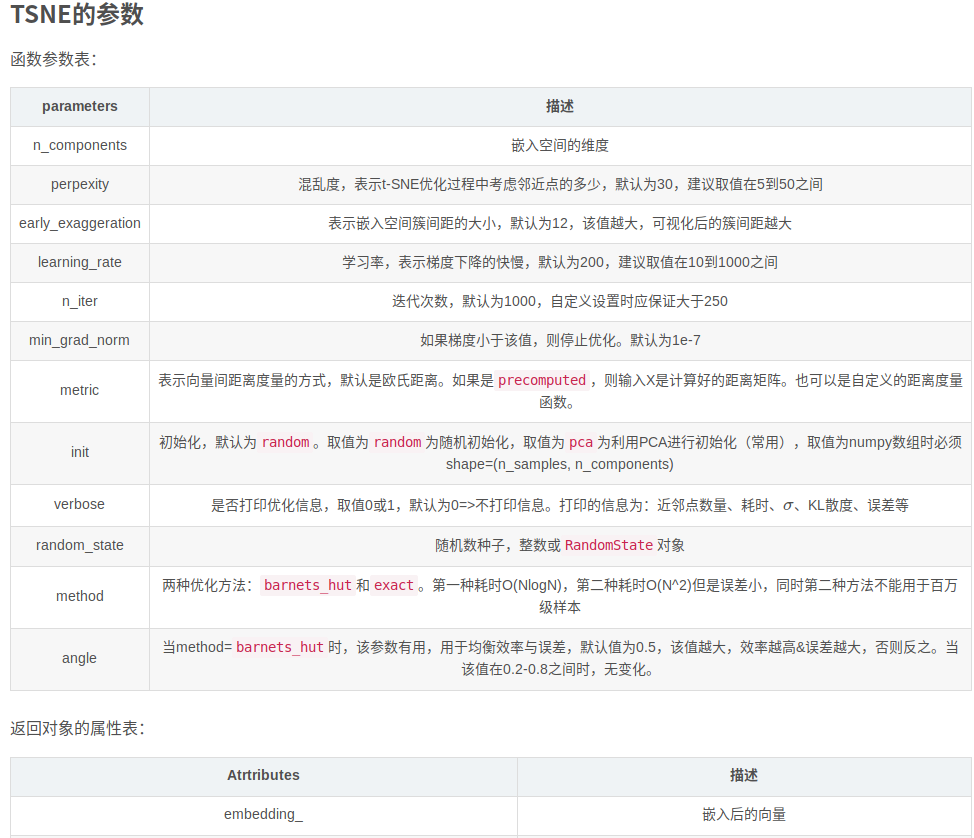

17 matplotlib知识：FontProperties添加中文字体

参考资料

【说明】

在默认状态下，matplotlb无法在图表中使用中文。

使用matplotlib的字体管理器指定字体文件

matplotlib中有一个字体管理器——matplotlib.Font_manager,通过该管理器的方法——matplotlib.Font_manager.FontProperties(fname)可以指

定一个ttf字体文件作为图表使用的字体。这样,只要我们传入Unicode字符串，我们就可以想用什么字体就用什么字体了。

【代码】

myfont = font_manager.FontProperties(fname='/home/dyy/Downloads/font163/simhei.ttf')