Enhancing Vision with Convolutional Neural Networks

参考：Ubuntu 16 安装TensorFlow及Jupyter notebook 安装TensorFlow。

本篇博客翻译来自 Introduction to TensorFlow for Artificial Intelligence, Machine Learning, and Deep Learning

仅供学习、交流等非盈利性质使用！！！

1. convolutions and pooling （卷积和池化）

在进行图像处理的过程中，经常会使用滤波器矩阵（Filter）来对原始图片进行处理，而这个过程就是卷积（convolutions）。
如下图所示：

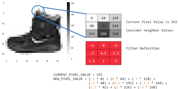
在上图中，针对其中的一个像素点，应用滤波器矩阵（图中给出的矩阵是随机定义的一个矩阵），那么卷积就是针对每个像素点，考虑其上下左右、左上下、右上下的邻居像素点，和滤波器矩阵对应点相乘得到新的像素点，这个转换过程就叫做卷积。

应用卷积可以具有特殊意义，如下两个图：

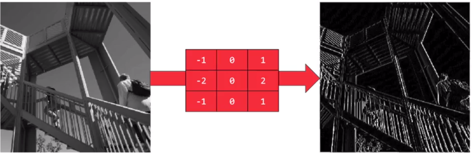
应用滤波器，可以把纵向特征明显化（即垂直特征明显）；

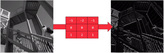
而应用这个滤波器，则可以把横向特征明显化（即水平特征明显）；

关于图像的卷积意义，推荐这篇博客：理解图像卷积操作的意义

池化：简单理解，就是图片的压缩，即把原始比如128*128像素的图片压缩成28*28的图片。

一个简单的例子，如下图：

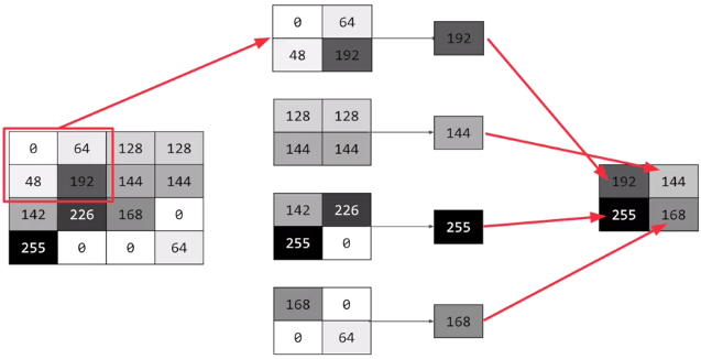
在图中，一个4*4像素的图片，被压缩为2*2的图片。其做法是：每次处理4个像素，找到其最大的像素进行返回。当然这只是其中的一种池化方法，你也可以针对4个像素进行求均值然后返回也可以。

2.实现卷积和池化

之前的代码：

model = tf.keras.models.Sequential([ 
    tf.keras.layers.Flatten(), 
    tf.keras.layers.Dense(128, activation=tf.nn.relu),
    tf.keras.layers.Dense(10, activation=tf.nn.softmax)])

在这个代码基础上，如何修改，可以添加卷积和池化层呢？
如下代码所示：

model = tf.keras.models.Sequential([
	tf.keras.layers.Conv2D(64,(3,3), activation='relu',input_shape=(28,28,1)),
	tf.keras.layers.MaxPooling2D(2,2),
	tf.keras.layers.Conv2D(64,(3,3),activation='relu'),
	tf.keras.layers.MaxPooling2D(2,2),
	tf.keras.layers.Flatten(), 
    tf.keras.layers.Dense(128, activation=tf.nn.relu), 
    tf.keras.layers.Dense(10, activation=tf.nn.softmax)
])

从代码中可看成：

最后三行是和之前一样的；
第二行，定义了一个卷积层（Conv2D)，这个卷积层有64个滤波器矩阵，每个矩阵是一个3*3的矩阵，activation是relu（会丢弃负值），而input_shape中的值是（28,28,1）,前面的28,28是图片的大小，而最后一个代表的是像素点的值，即图片是灰度图；
第二行的卷积层中的64个滤波器矩阵里面的值，最开始是随机的，随着训练的推进，这些值会被改变，而改变的方向则是使得最终预测效果较好的方向。
第三行是一个池化层，MaxPooling意味着最大值保留，同时池化的大小是(2,2),那么一次会处理4个像素点；
第四、五行继续添加了一个卷积层和池化层；
当一个图片经过2个卷积、池化层后，即叨叨Flatten时，图片会被缩小；
缩小的图片，其实指的是对于目标变量更有话语权的特征被筛选出来；

通过下面的代码可以查看构造的模型：

model.summary()

那么，上面构造的模型的summary是什么呢？如下所示：

_________________________________________________________________
Layer (type)                 Output Shape              Param #   
=================================================================
conv2d (Conv2D)              (None, 26, 26, 64)        640       
_________________________________________________________________
max_pooling2d (MaxPooling2D) (None, 13, 13, 64)        0         
_________________________________________________________________
conv2d_1 (Conv2D)            (None, 11, 11, 64)        36928     
_________________________________________________________________
max_pooling2d_1 (MaxPooling2 (None, 5, 5, 64)          0         
_________________________________________________________________
flatten (Flatten)            (None, 1600)              0         
_________________________________________________________________
dense (Dense)                (None, 128)               204928    
_________________________________________________________________
dense_1 (Dense)              (None, 10)                1290      
=================================================================
Total params: 243,786
Trainable params: 243,786
Non-trainable params: 0

从上面的数据结果可以看出:

第一层卷积输出的大小是26*26*64 ,这是什么意思呢？

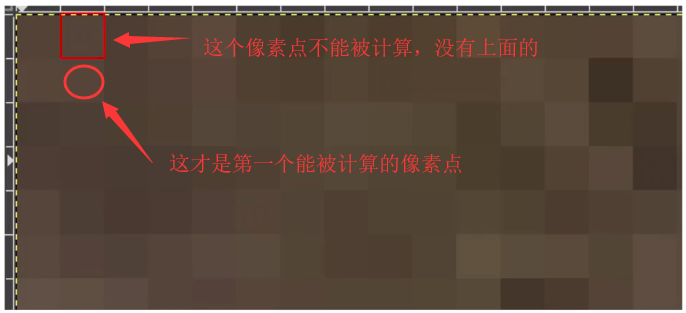
首先，一个28*28的图片数据经过卷积层的滤波器矩阵后，其图片变为26*26的大小。由于滤波器大小是3*3，所以原始28*28的图像的最外面的一圈像素点是不能被计算的。这样上下左右就会各少一个像素点，所以得到的是26*26的图片。

所以，如果滤波器是5*5，那么输出是多少呢？（应该是24*24，会少4个像素点）。

其次，64代表64个滤波器，那么一个图片就会输出64个新的图片。

第一个池化层，由于其大小是2*2，所以会把4个像素点变成一个，所以26*26的像素点，会变成13*13。
第二个卷积层是类似的，像素会减小2，所以是11*11.
第二个池化层，会把输入像素减半，即变成5*5 。
Flatten层的输入为什么是1600？ 1600 = 5*5*64，即把64个子图的所有像素点展平，作为Flatten的输入。

3. 使用卷积优化Fashion Mnist数据识别模型

之前的训练代码：

import tensorflow as tf
mnist = tf.keras.datasets.fashion_mnist
(training_images, training_labels), (test_images, test_labels) = mnist.load_data()
training_images=training_images / 255.0
test_images=test_images / 255.0
model = tf.keras.models.Sequential([
  tf.keras.layers.Flatten(),
  tf.keras.layers.Dense(128, activation=tf.nn.relu),
  tf.keras.layers.Dense(10, activation=tf.nn.softmax)
])
model.compile(optimizer='adam', loss='sparse_categorical_crossentropy', metrics=['accuracy'])
model.fit(training_images, training_labels, epochs=5)

test_loss = model.evaluate(test_images, test_labels)

执行完成后，可以得到训练集和测试集的误差及正确率，如下：

Epoch 1/5
60000/60000 [==============================] - 20s 340us/sample - loss: 0.4971 - acc: 0.8251
Epoch 2/5
60000/60000 [==============================] - 18s 306us/sample - loss: 0.3769 - acc: 0.8643
Epoch 3/5
60000/60000 [==============================] - 18s 292us/sample - loss: 0.3389 - acc: 0.8759
Epoch 4/5
60000/60000 [==============================] - 17s 291us/sample - loss: 0.3154 - acc: 0.8850
Epoch 5/5
60000/60000 [==============================] - 14s 230us/sample - loss: 0.2971 - acc: 0.8921
10000/10000 [==============================] - 2s 151us/sample - loss: 0.3676 - acc: 0.8657

改进后的代码，如下：

import tensorflow as tf
print(tf.__version__)
mnist = tf.keras.datasets.fashion_mnist
(training_images, training_labels), (test_images, test_labels) = mnist.load_data()
training_images=training_images.reshape(60000, 28, 28, 1)
training_images=training_images / 255.0
test_images = test_images.reshape(10000, 28, 28, 1)
test_images=test_images/255.0
model = tf.keras.models.Sequential([
  tf.keras.layers.Conv2D(64, (3,3), activation='relu', input_shape=(28, 28, 1)),
  tf.keras.layers.MaxPooling2D(2, 2),
  tf.keras.layers.Conv2D(64, (3,3), activation='relu'),
  tf.keras.layers.MaxPooling2D(2,2),
  tf.keras.layers.Flatten(),
  tf.keras.layers.Dense(128, activation='relu'),
  tf.keras.layers.Dense(10, activation='softmax')
])
model.compile(optimizer='adam', loss='sparse_categorical_crossentropy', metrics=['accuracy'])
model.summary()
model.fit(training_images, training_labels, epochs=5)
test_loss = model.evaluate(test_images, test_labels)

其结果如下：

Epoch 1/5
60000/60000 [==============================] - 216s 4ms/sample - loss: 0.4520 - acc: 0.8356
Epoch 2/5
60000/60000 [==============================] - 196s 3ms/sample - loss: 0.2985 - acc: 0.8904
Epoch 3/5
60000/60000 [==============================] - 208s 3ms/sample - loss: 0.2525 - acc: 0.9070
Epoch 4/5
60000/60000 [==============================] - 211s 4ms/sample - loss: 0.2236 - acc: 0.9172
Epoch 5/5
60000/60000 [==============================] - 201s 3ms/sample - loss: 0.1953 - acc: 0.9265
10000/10000 [==============================] - 9s 935us/sample - loss: 0.2658 - acc: 0.9051

通过上面的代码及其运行情况，可以得到：

使用优化后的代码，会比之前的代码运行更慢，因为其会涉及把图片进过两次卷积和池化，并且进行64个图片操作；
使用优化后的代码后，明显感觉到其在训练集、验证集的效果会更好。

4. 可视化卷积结果

本节主要是卷积结果的可视化，具体指的是：获取上面的模型，然后同时选择多个图片，以及一个卷积（滤波器矩阵），看模型的四层（第一次卷积、第一次池化、第二次卷积、第二次池化）的输出效果。

先查看测试数据的部分结果：

print(test_labels[:100])

输出为：

[9 2 1 1 6 1 4 6 5 7 4 5 7 3 4 1 2 4 8 0 2 5 7 9 1 4 6 0 9 3 8 8 3 3 8 0 7
 5 7 9 6 1 3 7 6 7 2 1 2 2 4 4 5 8 2 2 8 4 8 0 7 7 8 5 1 1 2 3 9 8 7 0 2 6
 2 3 1 2 8 4 1 8 5 9 5 0 3 2 0 6 5 3 6 7 1 8 0 1 4 2]

从上面的结果来看下标为0,23，28的图片都是9，也就是shoes，那么一般情况下，卷积可以针对同一类的图片，能发现其共同的特征，使用下面代码：

#%matplotlib
import matplotlib.pyplot as plt
f, axarr = plt.subplots(3,4)
FIRST_IMAGE=0 # 第一个图片下标
SECOND_IMAGE=23# 第二个图片下标
THIRD_IMAGE=28# 第三个图片下标
CONVOLUTION_NUMBER = 1 # 第1个卷积 ,调整卷积为1,2,6 ，可以看到不同图片
from tensorflow.keras import models
layer_outputs = [layer.output for layer in model.layers]
activation_model = tf.keras.models.Model(inputs = model.input, outputs = layer_outputs)
for x in range(0,4):
    f1 = activation_model.predict(test_images[FIRST_IMAGE].reshape(1, 28, 28, 1))[x]
    axarr[0,x].imshow(f1[0, : , :, CONVOLUTION_NUMBER], cmap='inferno')
    axarr[0,x].grid(False)
    f2 = activation_model.predict(test_images[SECOND_IMAGE].reshape(1, 28, 28, 1))[x]
    axarr[1,x].imshow(f2[0, : , :, CONVOLUTION_NUMBER], cmap='inferno')
    axarr[1,x].grid(False)
    f3 = activation_model.predict(test_images[THIRD_IMAGE].reshape(1, 28, 28, 1))[x]
    axarr[2,x].imshow(f3[0, : , :, CONVOLUTION_NUMBER], cmap='inferno')
    axarr[2,x].grid(False)

调整 CONVOLUTION_NUMBER分别为1,2,6，即可看到如下所示图片：

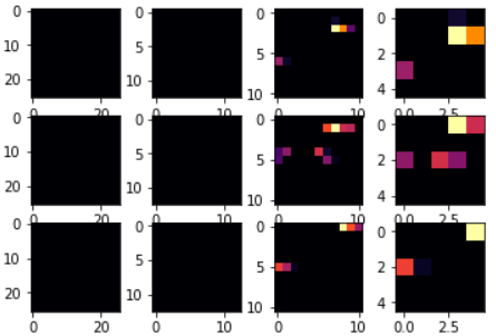
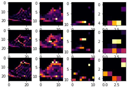
从图片中可以看到：

图片像素从最开始的28*28，变为26*26， -> 13*13 , -> 11*11 ,-> 5*5;
明显可以看出当CONVOLUTION_NUMBER为2时，其特征区分的最好（就3个对比来说）；

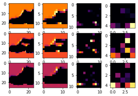
使用CONVOLUTION_NUMBER为2，并且调整第二个图片的下标为2，那么可以得到如下图：

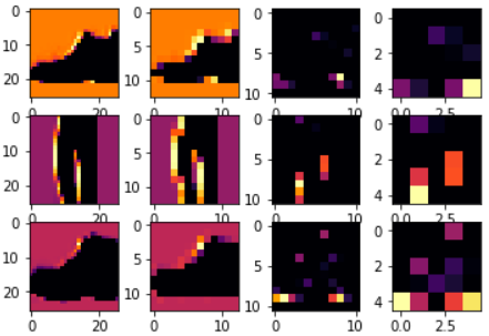
从图上可以看出，使用CONVOLUTION_NUMBER为2的滤波器矩阵，对图片的分类效果比较好，能较明显的区分鞋子和裤子。

5. 纯Python理解卷积和池化

使用如下代码，引入图片：

#%matplotlib
import cv2
import numpy as np
from scipy import misc
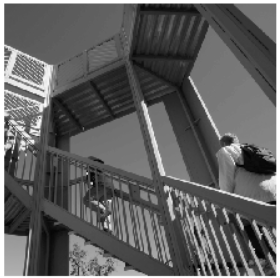
i = misc.ascent()

import matplotlib.pyplot as plt
plt.grid(False)
plt.gray()
plt.axis('off')
plt.imshow(i)
plt.show()

图片如下：

获取图片大小：

i_transformed = np.copy(i)
size_x = i_transformed.shape[0]
size_y = i_transformed.shape[1]

定义3*3 filter：

# This filter detects edges nicely
# It creates a convolution that only passes through sharp edges and straight
# lines.

#Experiment with different values for fun effects.
#filter = [ [0, 1, 0], [1, -4, 1], [0, 1, 0]]

# A couple more filters to try for fun!
filter = [ [-1, -2, -1], [0, 0, 0], [1, 2, 1]]
#filter = [ [-1, 0, 1], [-2, 0, 2], [-1, 0, 1]]

# If all the digits in the filter don't add up to 0 or 1, you 
# should probably do a weight to get it to do so
# so, for example, if your weights are 1,1,1 1,2,1 1,1,1
# They add up to 10, so you would set a weight of .1 if you want to normalize them
weight  = 1

应用卷积：

for x in range(1,size_x-1):
  for y in range(1,size_y-1):
      convolution = 0.0
      convolution = convolution + (i[x - 1, y-1] * filter[0][0])
      convolution = convolution + (i[x, y-1] * filter[0][1])
      convolution = convolution + (i[x + 1, y-1] * filter[0][2])
      convolution = convolution + (i[x-1, y] * filter[1][0])
      convolution = convolution + (i[x, y] * filter[1][1])
      convolution = convolution + (i[x+1, y] * filter[1][2])
      convolution = convolution + (i[x-1, y+1] * filter[2][0])
      convolution = convolution + (i[x, y+1] * filter[2][1])
      convolution = convolution + (i[x+1, y+1] * filter[2][2])
      convolution = convolution * weight
      if(convolution<0):
        convolution=0
      if(convolution>255):
        convolution=255
      i_transformed[x, y] = convolution

查看卷积后的结果：

# Plot the image. Note the size of the axes -- they are 512 by 512
plt.gray()
plt.grid(False)
plt.imshow(i_transformed)
#plt.axis('off')
plt.show()

得到的图如下：

应用池化：

new_x = int(size_x/2)
new_y = int(size_y/2)
newImage = np.zeros((new_x, new_y))
for x in range(0, size_x, 2):
    for y in range(0, size_y, 2):
        pixels = []
        pixels.append(i_transformed[x, y])
        pixels.append(i_transformed[x+1, y])
        pixels.append(i_transformed[x, y+1])
        pixels.append(i_transformed[x+1, y+1])
        pixels.sort(reverse=True)
        newImage[int(x/2),int(y/2)] = pixels[0]

# Plot the image. Note the size of the axes -- now 256 pixels instead of 512
plt.gray()
plt.grid(False)
plt.imshow(newImage)
#plt.axis('off')
plt.show()

查看结果：

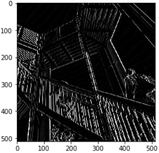
从结果可以看出，图片的一些特征是被强化的。

6. 测验：

第 1 个问题
What is a Convolution?

a. A technique to filter out unwanted images
b. A technique to make images bigger
c. A technique to make images smaller
d. A technique to isolate features in images

第 2 个问题
What is a Pooling?

a. A technique to isolate features in images
b. A technique to combine pictures
c. A technique to reduce the information in an image while maintaining features
d. A technique to make images sharper

第 3 个问题
How do Convolutions improve image recognition?

a. They make the image smaller
b. They make processing of images faster
c. They make the image clearer
d. They isolate features in images

第 4 个问题
After passing a 3x3 filter over a 28x28 image, how big will the output be?

a. 28x28
b. 25x25
c. 26x26
d. 31x31

第 5 个问题
After max pooling a 26x26 image with a 2x2 filter, how big will the output be?

a. 26x26
b. 28x28
c. 13x13
d. 56x56

第 6 个问题
Applying Convolutions on top of our Deep neural network will make training:

a. It depends on many factors. It might make your training faster or slower, and a poorly designed Convolutional layer may even be less efficient than a plain DNN!
b. Stay the same
c. Faster
d. Slower

 My Guess:
    1. d
    2. c
    3. d
    4.c
    5. c
    6. a

7. 额外练习：

针对MNIST数据构建的模型进行优化，同时满足如下要求：

提升正确率到99.8%+；
只能使用一个卷积层和一个池化层；
当达到99.8%+的正确率后，立即停止训练（正常情况下20步骤内可以达到），并打印Reached 99.8% accuracy so cancelling training!；

下面是提示代码：

import tensorflow as tf

# YOUR CODE STARTS HERE

# YOUR CODE ENDS HERE

mnist = tf.keras.datasets.mnist
(training_images, training_labels), (test_images, test_labels) = mnist.load_data()

# YOUR CODE STARTS HERE

# YOUR CODE ENDS HERE

model = tf.keras.models.Sequential([
    # YOUR CODE STARTS HERE

    # YOUR CODE ENDS HERE
])

# YOUR CODE STARTS HERE

# YOUR CODE ENDS HERE

Answer

Code Download Here

Coursera TensorFlow 基础课程-week3