1.Python 数据类型
Python 内置的常用数据类型共有6中:
数字(Number)、布尔值(Boolean)、字符串(String)、元组(Tuple)、列表(List)、字典(Dictionary)。
数字:常用的数字类型包括整型数(Integer)、长整型(Long)、浮点数(Float)、复杂型数(Complex)。
10、100、-100都是整型数;-0.1、10.01是浮点数。
布尔值:True代表真,False代表假。
字符串:在Python里,字符串的表示使用成对的英文单引号,双引号进行表示,‘abc’或“123”。
元组:使用一组小括号()表示,(1,‘abc’,0.4)是一个包含三个元素的元组。假设上例的这个元组叫做t,那么t[0]=1,t[1]='abc'。默认索引的起始值为0,不是1。
列表:使用一对中括号[ ]来组织数据,[1,‘abc’,0.4]。需要注意的是Python允许在访问列表时同时修改列表里的数据,而元组则不然。
字典:包括多组键(key):值(value),Python使用大括号{ }来容纳这些键值对,{1:‘1’,‘abc’:0.1,0.4:80},假设上例字典为变量d,那么d[1]='1',d['abc']=0.1
2.Python 流程控制
比较常见的包括分支语句(if)和循环控制(for)
分支语句语法结构:
if布尔值/表达式:
else:
或者
if布尔值/表达式:
elif布尔值/表达式:
else:
代码1:分支语句代码样例:
=====》
b=True
if b:
print("It's True!")
else:
print('It's False!")
=====》
It's True!
=====》
b=False
c=True
if b:
print("b is True!")
elif c:
print('c is True!")
else:
print("both are False")
=====》
c is True!
循环控制语法结构:
for 临时变量 in 可遍历数据结构(列表、元组、字典)
执行语句
代码2:循环语句代码样例:
=====》
d={1:'1','abc':0.1,0.4:80}
for k in d:
print(k,":",d[k])
=====》
1:1
abc:0.1
0.4:80
1.3 Python函数模块设计
Python采用def关键字来定义一个函数:
代码3:函数定义和调用代码样例:
=====》
def foo(x):
return x**2
print(foo(8.0))
=====》
64.0
1.4 Python编程库(包)的导入
代码4:程序库/工具包导入代码示例
=====》
import math
#调用math包下的函数exp求自然指数
print(math.exp(2))
#2.从(from)math工具包里指定导入exp函数
from math import exp
print(exp(2))
#3.从(from)math工具包里指定导入exp函数,并且对exp重新命名为ep
from math import exp as ep
print(ep(2))
=====》
7.38905609893065
7.38905609893065
7.38905609893065
1.5 Python基础综合实践
代码5:良/恶性乳腺癌肿瘤预测代码样例
=====》
import pandas as pd
#调用pandas工具包的read_csv函数/模块,传入训练文件地址参数,获得返回的数据并且存至变量df_train
df_train=pd.read_csv('breast-cancer-train.csv')
#调用pandas工具包的read_csv函数/模块,传入测试文件地址参数,获得返回的数据并且存至变量df_test
df_test=pd.read_csv('breast-cancer-test.csv')
#选取‘肿块厚度’(Clump Thickness)与‘细胞大小’(Cell Size)作为特征,构建测试集中的正负分类样本
df_test_negative=df_test.loc[df_test['Type']==0][['Clump Thickness','Cell Size']]
df_test_positive=df_test.loc[df_test['Type']==1][['Clump Thickness','Cell Size']]
#导入matplotlib工具包中pyplot并命名为plt
import matplotlib.pyplot as plt
#matplotlib.pyplot.scatter(x,y,s=None,c=None,marker=None)
#x,y接收array。表示x轴和y轴对应的数据。无默认
#s接收数值或者一维的array。指定点的大小,若传入一维array,则表示每个点的大小。默认为None
#c接收颜色或者一维的array。指定点的颜色,若传入一维array,则表示每个点的颜色。默认为None
#marker接收特定string。表示绘制的点的类型。默认为None
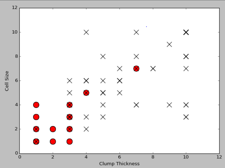
#绘制良性肿瘤样本点,标记为红色的o
plt.scatter(df_test_negative['Clump Thickness'],df_test_negative['Cell Size'],marker='o',s=200,c='red')
#绘制恶性肿瘤样本点,标记为黑色的x
plt.scatter(df_test_positive['Clump Thickness'],df_test_positive['Cell Size'],marker='x',s=150,c='black')
#绘制x,y轴的说明
plt.xlabel('Clump Thickness')
plt.ylabel('Cell Size')
#显示图
plt.show()
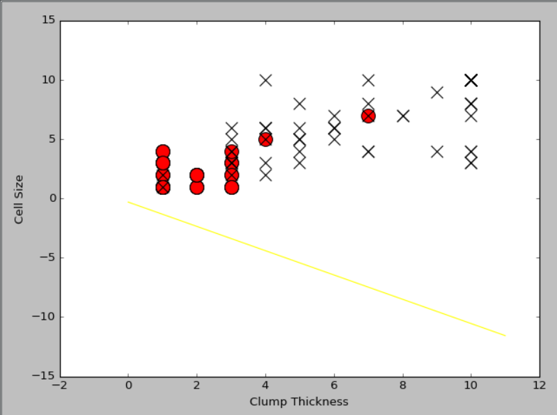
import numpy as np
#利用numpy中的random函数随机采样直线的截距和系数
intercept=np.random.random([1])
# print(intercept)#[0.79195932]
coef=np.random.random([2])
# print(coef)#[0.37965899 0.47387532]
lx=np.arange(0,12)
# print(lx)#[ 0 1 2 3 4 5 6 7 8 9 10 11]
ly=(-intercept-lx*coef[0])/coef[1]
# print(ly)
# [-1.09996728 -1.60387435 -2.10778142 -2.61168849 -3.11559556 -3.61950262
# # -4.12340969 -4.62731676 -5.13122383 -5.6351309 -6.13903797 -6.64294503]
#绘制一条随机直线
plt.plot(lx,ly,c='yellow')
plt.scatter(df_test_negative['Clump Thickness'],df_test_negative['Cell Size'],marker='o',s=200,c='red')
plt.scatter(df_test_positive['Clump Thickness'],df_test_positive['Cell Size'],marker='x',s=150,c='black')
plt.xlabel('Clump Thickness')
plt.ylabel('Cell Size')
plt.show()
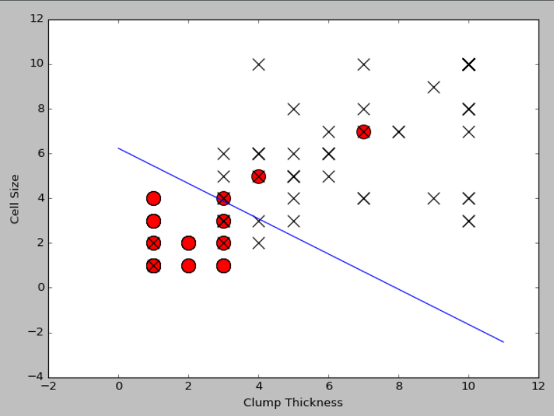
#导入sklearn中的逻辑斯蒂回归分类器
from sklearn.linear_model import LogisticRegression
lr=LogisticRegression()
#使用前10条训练样本学习直线的系数和截距
lr.fit(df_train[['Clump Thickness','Cell Size']][:10],df_train['Type'][:10])
print('Testing accuracy (10 training samples):',lr.score(df_test[['Clump Thickness','Cell Size']],df_test['Type']))
intercept=lr.intercept_
coef=lr.coef_[0,:]
#原本这个分类面应该是lx*coef[0]+ly*coef[1]+intercept=0,映射到2维平面上之后,应该是:
ly=(-intercept-lx*coef[0])/coef[1]
plt.plot(lx,ly,c='green')
plt.scatter(df_test_negative['Clump Thickness'],df_test_negative['Cell Size'],marker='o',s=200,c='red')
plt.scatter(df_test_positive['Clump Thickness'],df_test_positive['Cell Size'],marker='x',s=150,c='black')
plt.xlabel('Clump Thickness')
plt.ylabel('Cell Size')
plt.show()

lr=LogisticRegression()
#使用所有的训练样本学习直线的系数和截距
lr.fit(df_train[['Clump Thickness','Cell Size']],df_train['Type'])
print('Testing accuracy (all training samples):',lr.score(df_test[['Clump Thickness','Cell Size']],df_test['Type']))
intercept=lr.intercept_
coef=lr.coef_[0,:]
#原本这个分类面应该是lx*coef[0]+ly*coef[1]+intercept=0,映射到2维平面上之后,应该是:
ly=(-intercept-lx*coef[0])/coef[1]
plt.plot(lx,ly,c='blue')
plt.scatter(df_test_negative['Clump Thickness'],df_test_negative['Cell Size'],marker='o',s=200,c='red')
plt.scatter(df_test_positive['Clump Thickness'],df_test_positive['Cell Size'],marker='x',s=150,c='black')
plt.xlabel('Clump Thickness')
plt.ylabel('Cell Size')
plt.show()
Testing accuracy (all training samples): 0.9371428571428572