神经网络 pytorch 分类二维矩阵图像和一维向量的方法

在网上找资料的过程中，发现并没有特别细致的讲解分类图像和分类一维向量的做法，导致我捅咕了有几天才弄明白，可能使我比较菜吧......现在在这里记录一下。

首先需要明确，前文我们已经讲解了包装数据集的方法，但是注意，无论是图像还是向量数据，都是有固定格式的，因为我们在做卷积的时候有数据格式要求。使用的时候我们必须将自己的数据变换为指定的格式，而变换的方法无非numpy.array torch.from_numpy 香江列表转换为矩阵，再从矩阵转换为tensor，这其中的操作就是矩阵的操作，在上一篇中简单有一个例子，简单了解一下就可以，注意以下问题

矩阵维度必须满足卷积的输入
label是有数据类型要求的，tensor可以直接使用.int() .long()等方法就行转换类型
变换时，可以使用矩阵的赋值和循环操作结合，完成指定格式的数据构建具体看前一篇（神经网络 pytorch 数据集读取（自动读取数据集，手动读取自己的数据））

基础

数据分为两部分：原始数据，数据标签

图像数据要求的格式为【样本序号，维度，尺寸w，尺寸h】、

向量要求是【样本序号，维度，长度】

这里的维度代表的是。。。。举个例子一张彩色图像可以分为三个RGB通道

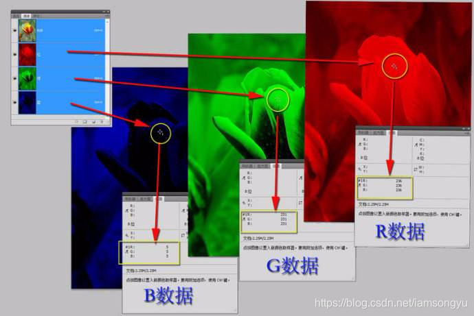
所以一张图像读取进来的数据是【维度，尺寸w，尺寸h】，在加上组成数据集的样本维度，就变为了【样本序号，维度，尺寸w，尺寸h】。

而对于一维向量来说，由于没有宽高，只有长度，所以就变为了

【样本序号，维度，长度】

实验

首先是图像的二维数据测试

conv1 = nn.Conv2d(3, 6, 5)
conv1 = nn.Conv2d(in_channels=3, out_channels=6, kernel_size=5)
这是二维卷积函数，可以看到输入要求3维度 输出6图 核大小5维

在卷积中使用的是batch分组进行处理的，所以在图像的基础上，我们还需要再有一个维度

【batch，维度，尺寸w，尺寸h】，注意如果使用数据集的话，batch是不需要我们管的

我们创建数据
conv1 = nn.Conv2d(3, 6, 5)
input = torch.randn((3,15,15)) #这是一个图像的三维 尺寸
conv1(input)
# Expected 4-dimensional input for 4-dimensional weight [6, 3, 5, 5], but got input of size [3, 15, 15] instead
# 要求输入为四维 我们手动创建一个样本集
input = torch.randn((5,3,15,15))  # 五张图像 三维 尺寸
conv1(input)
tensor([[[[-0.3294, -0.4139, -0.2850,  ...,  1.3533, -0.6759,  0.1333],
          [ 0.3084,  0.1447, -0.1788,  ...,  0.9002,  0.2388,  0.9239],
          [ 0.0672,  0.2839,  1.3691,  ..., -0.1531, -1.0619, -1.0429],
          ...,
          [-0.2464,  0.4404,  0.6528,  ...,  0.4497, -0.2516, -0.1859],
          [-0.3036,  0.1986,  0.6850,  ..., -0.1474, -0.3568, -0.1044],
          [ 0.0053,  0.4006, -0.2252,  ..., -0.0466,  0.0872,  0.0611]],
         [[ 1.2968, -0.4136, -0.2831,  ..., -0.1858, -0.9087,  0.5293],
          [ 0.4907,  0.6914,  0.3149,  ...,  0.3644,  0.5656, -0.8398],
          [ 0.1517, -0.1849, -0.0562,  ..., -0.5456, -0.4508, -0.6404],
          ..., 省略了
          ...,
          [-0.0307,  0.5376, -0.8060,  ..., -0.1753, -0.7272, -0.8466],
          [-0.2170, -0.2148, -0.5993,  ...,  0.0340,  0.3307,  0.0338],
          [ 0.3770,  0.5640,  0.0672,  ..., -0.1321, -0.7813,  0.2787]]]],
       grad_fn=<ThnnConv2DBackward>)

对于一维的学习来说，输入是三维的，【样本序号，维度，长度】，继续试验一下

conv1 = nn.Conv1d(in_channels=2, out_channels=5, kernel_size=3)
# 要求输入为二通道
input = torch.randn((4,2,12))
# 四个样本 二通道 长度12
conv1(input)

tensor([[[ 0.5587,  0.6236, -0.9632,  0.3872, -0.0721,  0.3657, -0.1207,
          -0.0946,  0.3658, -0.3244],
         [ 0.2307, -0.2126, -1.2743, -0.4488, -0.2530, -0.0273, -0.7402,
           0.0616, -0.9748, -0.6859],
         [-0.7817, -0.3664, -1.1842, -0.7359,  0.4219,  0.6737, -0.1494,
          -0.0247, -0.2200, -0.1169],
         [ 0.4604, -0.6700,  0.3021,  0.6606,  2.2227,  0.3312,  0.5341,
           0.8271, -0.7024,  0.7300],
         [ 0.0626, -0.4945,  0.9787,  0.0997,  0.4146, -0.6470,  0.6352,
          -0.0103, -0.0971,  0.6143]],
         ............. 省略
        [[-0.0005,  0.6630,  0.2095,  0.4185,  0.0364,  0.8880,  0.1139,
           0.3172, -0.1049,  0.1099],
         [-0.2716,  0.0824, -0.5943,  0.0037, -0.6148,  0.3952, -0.1688,
          -0.3591, -0.6956, -0.5202],
         [-0.7579, -1.2024, -1.1410, -0.3624, -1.0320, -0.2396, -0.5218,
          -0.7605, -0.4535, -0.6400],
         [ 0.0183, -0.9959,  0.3437, -0.0709,  0.3040,  0.4322,  0.0317,
           0.1266, -0.0621,  0.7542],
         [ 0.3895, -0.4234,  0.6149, -0.4937,  0.5438, -0.4094, -0.0073,
           0.1984,  0.0270,  0.5017]]], grad_fn=<SqueezeBackward1>)

二维学习中，主要使用的是

self.conv1 = nn.Conv2d(in_channels=1, out_channels=5, kernel_size=7, stride=2, padding=1)

self.fc1 = nn.Linear(2432,512)

F.max_pool2d(self.conv1(x), 2)

一维

self.conv1 = nn.Conv1d(in_channels=1, out_channels=5, kernel_size=7, stride=2, padding=1)

self.fc1 = nn.Linear(2432,512)

F.max_pool1d(self.conv1(x), 2)

附录

下面的就是一些常用的可能的部分，每个都有很多种选择，但前提可定是需要知道它有......

其中激活函数包括多种，用于处理输出形式，规范等

torch.nn.functional.threshold(input, threshold, value, inplace=False)
torch.nn.functional.relu(input, inplace=False)
torch.nn.functional.hardtanh(input, min_val=-1.0, max_val=1.0, inplace=False)
torch.nn.functional.relu6(input, inplace=False)
torch.nn.functional.elu(input, alpha=1.0, inplace=False)
torch.nn.functional.leaky_relu(input, negative_slope=0.01, inplace=False)
torch.nn.functional.prelu(input, weight)
torch.nn.functional.rrelu(input, lower=0.125, upper=0.3333333333333333, training=False, inplace=False)
torch.nn.functional.logsigmoid(input)
torch.nn.functional.hardshrink(input, lambd=0.5)
torch.nn.functional.tanhshrink(input)
torch.nn.functional.softsign(input)
torch.nn.functional.softplus(input, beta=1, threshold=20)
torch.nn.functional.softmin(input)
torch.nn.functional.softmax(input)
torch.nn.functional.softshrink(input, lambd=0.5)
torch.nn.functional.log_softmax(input)
torch.nn.functional.tanh(input)
torch.nn.functional.sigmoid(input)

常用的就是relu什么的，实际上种类很多，还有各种改进，具体的看这位大佬的吧

https://www.jianshu.com/p/68bd249327ce，列举了几种样式

优化器的话也是有上十种，基于基类 Optimizer

随机梯度下降算法 SGD算法 
torch.optim.SGD(params, lr=, momentum=0, dampening=0, weight_decay=0, nesterov=False)

平均随机梯度下降算法 ASGD算法
torch.optim.ASGD(params, lr=0.01, lambd=0.0001, alpha=0.75, t0=1000000.0, weight_decay=0)

AdaGrad算法
torch.optim.Adagrad(params, lr=0.01, lr_decay=0, weight_decay=0)

自适应学习率调整 Adadelta算法
torch.optim.Adadelta(params, lr=1.0, rho=0.9, eps=1e-06, weight_decay=0)

RMSprop算法
torch.optim.RMSprop(params, lr=0.01, alpha=0.99, eps=1e-08, weight_decay=0, momentum=0, centered=False)

自适应矩估计 Adam算法
torch.optim.Adam(params, lr=0.001, betas=(0.9, 0.999), eps=1e-08, weight_decay=0)

 Adamax算法（Adamd的无穷范数变种）
torch.optim.Adamax(params, lr=0.002, betas=(0.9, 0.999), eps=1e-08, weight_decay=0)

SparseAdam算法
torch.optim.SparseAdam(params, lr=0.001, betas=(0.9, 0.999), eps=1e-08)

L-BFGS算法
torch.optim.LBFGS(params, lr=1, max_iter=20, max_eval=None, tolerance_grad=1e-05, tolerance_change=1e-09, history_size=100, line_search_fn=None)

弹性反向传播算法 Rprop算法
torch.optim.Rprop(params, lr=0.01, etas=(0.5, 1.2), step_sizes=(1e-06, 50))

大佬的很详细
https://blog.csdn.net/shanglianlm/article/details/85019633

池化方法也有好几种

# https://blog.csdn.net/HowardWood/article/details/79508805
torch.nn.functional.avg_pool1d(input, kernel_size, stride=None, padding=0, ceil_mode=False, count_include_pad=True)
torch.nn.functional.avg_pool2d(input, kernel_size, stride=None, padding=0, ceil_mode=False, count_include_pad=True)
torch.nn.functional.max_pool1d(input, kernel_size, stride=None, padding=0, dilation=1, ceil_mode=False, return_indices=False)
torch.nn.functional.max_pool2d(input, kernel_size, stride=None, padding=0, dilation=1, ceil_mode=False, return_indices=False)
torch.nn.functional.max_unpool1d(input, indices, kernel_size, stride=None, padding=0, output_size=None)
torch.nn.functional.max_unpool2d(input, indices, kernel_size, stride=None, padding=0, output_size=None)
torch.nn.functional.lp_pool2d(input, norm_type, kernel_size, stride=None, ceil_mode=False)
torch.nn.functional.adaptive_max_pool1d(input, output_size, return_indices=False)
torch.nn.functional.adaptive_max_pool2d(input, output_size, return_indices=False)
torch.nn.functional.adaptive_avg_pool1d(input, output_size)
torch.nn.functional.adaptive_avg_pool2d(input, output_size)

神经网络 pytorch 分类二维矩阵图像和一维向量的方法

基础

实验

附录

猜你喜欢