1.OLS说明
最小二乘法。给定序列X(x1,x2...xn),y,估计一个向量A(a0,a1.a2....)令y'=a0+a1*x1+a2*x2+...+an*xn, 使得(y'-y)^2最小,计算A。
2.代码如下
来源《python机器学习实践指南》
import patsy
import statsmodels.api as sm
f = 'Rent ~ Zip + Beds'
y, X = patsy.dmatrices(f, su_lt_two, return_type='dataframe')
results = sm.OLS(y, X).fit()
print(results.summary())
结果如下:
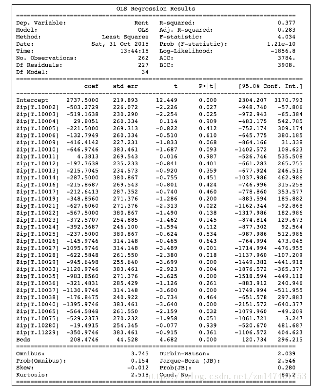
接下来一个一个说明
| 名称 | 值 | 说明 |
| 左边参数 | ||
| Dep. Variable | Rent | Which variable is the response in the model 输出Y变量的名称Rent |
| Model | OLS | What model you are using in the fit 使用的参数确定的模型OLS |
| Method | Least Squares |
How the parameters of the model were calculated 使用最小二乘法的方法确定参数 |
| Date | Sat,31 Oct 2015 | 日期 |
| Time | 13:44:15 | 时间 |
| No. Observations | 262 | The number of observations (examples) 样本数目 |
| DF Residuals | 227 | Degrees of freedom of the residuals. Number of observations - number of parameters 残差的自由度(等于 观测数(No. Observations)-参数数目(Df Model+1(常量参数))) 残差:指实际观察值与估计值(拟合值)之间的差 |
| Df Model: | 34 | 模型参数个数(不包含常量参数),对应于coef中的行数 |
| 右边参数 | ||
| R-squared | 0.377 | The coefficient of determination. A statistical measure of how well the regression line approximates the real data points 可决系数,说明估计的准确性 “可决系数”是通过数据的变化来表征一个拟合的好坏。由上面的表达式可以知道“确定系数”的正常取值范围为[0 1],越接近1,表明方程的变量对y的解释能力越强,这个模型对数据拟合的也较好 相关说明见下文 |
| Adj. R-squared |
0.283 | The above value adjusted based on the number of observations and the degrees-of-freedom of the residuals 修正方,见3.5 |
| F-statistic | 4.034 | A measure how significant the fit is. The mean squared error of the model divided by the mean squared error of the residuals |
| Prob (F-statistic) | ||
| Log-likelihood | ||
| AIC | Akaike Information Criterion AIC=2k+nln(SSR/n) |
|
| BIC |
https://blog.datarobot.com/ordinary-least-squares-in-python
3.统计学相关参数:
SSE(和方差、误差平方和):The sum of squares due to error
MSE(均方差、方差):Mean squared error
RMSE(均方根、标准差):Root mean squared error
R-square(确定系数):Coefficient of determination
Adjusted R-square:Degree-of-freedom adjusted coefficient of determination
下面我对以上几个名词进行详细的解释下,相信能给大家带来一定的帮助!!
一、SSE(和方差)
该统计参数计算的是拟合数据和原始数据对应点的误差的平方和,计算公式如下
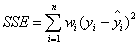
SSE越接近于0,说明模型选择和拟合更好,数据预测也越成功。接下来的MSE和RMSE因为和SSE是同出一宗,所以效果一样
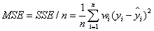
二、MSE(均方差)
该统计参数是预测数据和原始数据对应点误差的平方和的均值,也就是SSE/n,和SSE没有太大的区别,计算公式如下
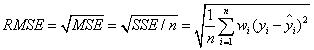
三、RMSE(均方根)
该统计参数,也叫回归系统的拟合标准差,是MSE的平方根,就算公式如下
在这之前,我们所有的误差参数都是基于预测值(y_hat)和原始值(y)之间的误差(即点对点)。从下面开始是所有的误差都是相对原始数据平均值(y_ba)而展开的(即点对全)!!!
四、R-square(确定系数)
在讲确定系数之前,我们需要介绍另外两个参数SSR和SST,因为确定系数就是由它们两个决定的
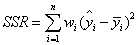
(1)SSR:Sum of squares of the regression,即预测数据与原始数据均值之差的平方和,公式如下
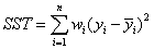
(2)SST:Total sum of squares,即原始数据和均值之差的平方和,公式如下
细心的网友会发现,SST=SSE+SSR,呵呵只是一个有趣的问题。而我们的“确定系数”是定义为SSR和SST的比值,故
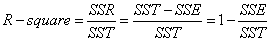
其实“确定系数”是通过数据的变化来表征一个拟合的好坏。由上面的表达式可以知道“确定系数”的正常取值范围为[0 1],越接近1,表明方程的变量对y的解释能力越强,这个模型对数据拟合的也较好
五、修正的公式(Adj. R-squared)
其中n是样本数量(No. Observations),p是模型中变量的个数(Df Model)。
我们知道在其他变量不变的情况下,引入新的变量,总能提高模型的。修正
就是相当于给变量的个数加惩罚项。
换句话说,如果两个模型,样本数一样,一样,那么从修正
的角度看,使用变量个数少的那个模型更优。使用修正
也算一种奥卡姆剃刀的实例。