https://scikit-learn.org/stable/auto_examples/model_selection/plot_roc_crossval.html
https://scikit-learn.org/stable/auto_examples/model_selection/plot_precision_recall.html
一,ROC
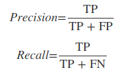
横轴:负正类率(false postive rate FPR)特异度,划分实例中所有负例占所有负例的比例;(1-Specificity)
负正类率(False Postive Rate)FPR: FP/(FP+TN),代表分类器预测的正类中实际负实例占所有负实例的比例。1-Specificity
纵轴:真正类率(true postive rate TPR)灵敏度,Sensitivity(正类覆盖率)
真正类率(True Postive Rate)TPR: TP/(TP+FN),代表分类器预测的正类中实际正实例占所有正实例的比例。
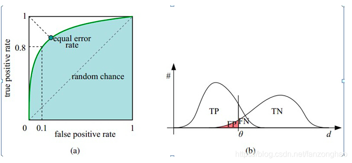
如下面这幅图,(a)图中实线为ROC曲线,线上每个点对应一个阈值。
横轴FPR:1-TNR,1-Specificity,FPR越大,预测正类中实际负类越多。
纵轴TPR:Sensitivity(正类覆盖率),TPR越大,预测正类中实际正类越多。
理想目标:TPR=1,FPR=0,即图中(0,1)点,故ROC曲线越靠拢(0,1)点,越偏离45度对角线越好,Sensitivity、Specificity越大效果越好。
假设已经得出一系列样本被划分为正类的概率,然后按照大小排序,下图是一个示例,图中共有20个测试样本,“Class”一栏表示每个测试样本真正的标签(p表示正样本,n表示负样本),“Score”表示每个测试样本属于正样本的概率。
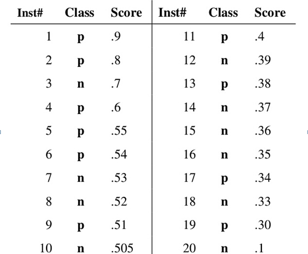
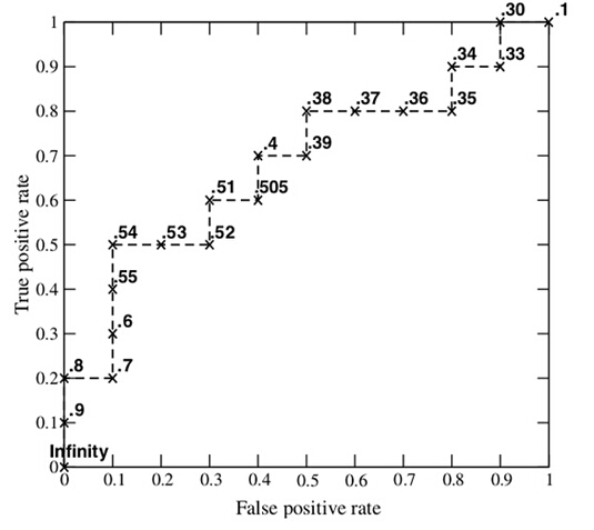
接下来,我们从高到低,依次将“Score”值作为阈值threshold,当测试样本属于正样本的概率大于或等于这个threshold时,我们认为它为正样本,否则为负样本。举例来说,对于图中的第4个样本,其“Score”值为0.6,那么样本1,2,3,4都被认为是正样本,因为它们的“Score”值都大于等于0.6,而其他样本则都认为是负样本。每次选取一个不同的threshold,我们就可以得到一组FPR和TPR,即ROC曲线上的一点。这样一来,我们一共得到了20组FPR和TPR的值,将它们画在ROC曲线的结果如下图:
AUC(Area under Curve):Roc曲线下的面积,介于0.1和1之间。Auc作为数值可以直观的评价分类器的好坏,值越大越好。
首先AUC值是一个概率值,当你随机挑选一个正样本以及负样本,当前的分类算法根据计算得到的Score值将这个正样本排在负样本前面的概率就是AUC值,AUC值越大,当前分类算法越有可能将正样本排在负样本前面,从而能够更好地分类。
为什么使用Roc和Auc评价分类器
既然已经这么多标准,为什么还要使用ROC和AUC呢?因为ROC曲线有个很好的特性:当测试集中的正负样本的分布变换的时候,ROC曲线能够保持不变。在实际的数据集中经常会出现样本类不平衡,即正负样本比例差距较大,而且测试数据中的正负样本也可能随着时间变化。下图是ROC曲线和Presision-Recall曲线的对比:

在上图中,(a)和(c)为Roc曲线,(b)和(d)为Precision-Recall曲线。
(a)和(b)展示的是分类其在原始测试集(正负样本分布平衡)的结果,(c)(d)是将测试集中负样本的数量增加到原来的10倍后,分类器的结果,可以明显的看出,ROC曲线基本保持原貌,而Precision-Recall曲线变化较大。
import numpy as np
from scipy import interp
import matplotlib.pyplot as plt

from sklearn import svm, datasets
from sklearn.metrics import roc_curve, auc
from sklearn.model_selection import StratifiedKFold

# #############################################################################
# Data IO and generation

# Import some data to play with
iris = datasets.load_iris()
X = iris.data
y = iris.target
X, y = X[y != 2], y[y != 2]
print('X.shape=',X.shape)
print('y.shape=',y.shape)
print(y)
n_samples, n_features = X.shape

# Add noisy features
random_state = np.random.RandomState(0)
X = np.hstack([X, random_state.randn(n_samples, 200 * n_features)])
print('X.shape=',X.shape)
# #############################################################################
# Classification and ROC analysis

# Run classifier with cross-validation and plot ROC curves
cv = StratifiedKFold(n_splits=6)
classifier = svm.SVC(kernel='linear', probability=True,
                     random_state=random_state)

tprs = []
aucs = []
mean_fpr = np.linspace(0, 1, 100)

i = 0
for train, test in cv.split(X, y):
    probas_ = classifier.fit(X[train], y[train]).predict_proba(X[test])
    print(probas_)
    print('probas_.shape=',probas_.shape)
    # Compute ROC curve and area the curve
    fpr, tpr, thresholds = roc_curve(y[test], probas_[:, 1])
    tprs.append(interp(mean_fpr, fpr, tpr))
    tprs[-1][0] = 0.0
    roc_auc = auc(fpr, tpr)
    aucs.append(roc_auc)
    plt.plot(fpr, tpr, lw=1, alpha=0.3,
             label='ROC fold %d (AUC = %0.2f)' % (i, roc_auc))

    i += 1
plt.plot([0, 1], [0, 1], linestyle='--', lw=2, color='r',
         label='Chance', alpha=.8)

mean_tpr = np.mean(tprs, axis=0)
mean_tpr[-1] = 1.0
mean_auc = auc(mean_fpr, mean_tpr)
std_auc = np.std(aucs)
plt.plot(mean_fpr, mean_tpr, color='b',
         label=r'Mean ROC (AUC = %0.2f $\pm$ %0.2f)' % (mean_auc, std_auc),
         lw=2, alpha=.8)

std_tpr = np.std(tprs, axis=0)
tprs_upper = np.minimum(mean_tpr + std_tpr, 1)
tprs_lower = np.maximum(mean_tpr - std_tpr, 0)
plt.fill_between(mean_fpr, tprs_lower, tprs_upper, color='grey', alpha=.2,
                 label=r'$\pm$ 1 std. dev.')

plt.xlim([-0.05, 1.05])
plt.ylim([-0.05, 1.05])
plt.xlabel('False Positive Rate')
plt.ylabel('True Positive Rate')
plt.title('Receiver operating characteristic example')
plt.legend(loc="lower right")
plt.show()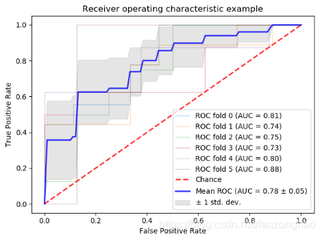
二,AP
PR曲线的横轴Recall也就是TPR,反映了分类器对正例的覆盖能力。而纵轴Precision的分母是识别为正例的数目,而不是实际正例数目。Precision反映了分类器预测正例的准确程度。那么,Precision-recall曲线反映了分类器对正例的识别准确程度和对正例的覆盖能力之间的权衡。AP就是PR曲线与X轴围成的图形面积。
from sklearn import svm, datasets
from sklearn.model_selection import train_test_split
import numpy as np

iris = datasets.load_iris()
X = iris.data
y = iris.target

# Add noisy features
random_state = np.random.RandomState(0)
n_samples, n_features = X.shape
X = np.hstack([X, random_state.randn(n_samples, 200 * n_features)])

# Limit to the two first classes, and split into training and test
X_train, X_test, y_train, y_test = train_test_split(X[y < 2], y[y < 2],
                                                    test_size=.5,
                                                    random_state=random_state)

# Create a simple classifier
classifier = svm.LinearSVC(random_state=random_state)
classifier.fit(X_train, y_train)
y_score = classifier.decision_function(X_test)
from sklearn.metrics import average_precision_score
average_precision = average_precision_score(y_test, y_score)

print('Average precision-recall score: {0:0.2f}'.format(
      average_precision))

from sklearn.metrics import precision_recall_curve
import matplotlib.pyplot as plt
from sklearn.utils.fixes import signature

precision, recall, _ = precision_recall_curve(y_test, y_score)

# In matplotlib < 1.5, plt.fill_between does not have a 'step' argument
step_kwargs = ({'step': 'post'}
               if 'step' in signature(plt.fill_between).parameters
               else {})
plt.step(recall, precision, color='b', alpha=0.2,
         where='post')
plt.fill_between(recall, precision, alpha=0.2, color='b', **step_kwargs)

plt.xlabel('Recall')
plt.ylabel('Precision')
plt.ylim([0.0, 1.05])
plt.xlim([0.0, 1.0])
plt.title('2-class Precision-Recall curve: AP={0:0.2f}'.format(
          average_precision))
plt.show()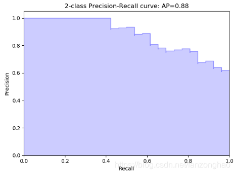
参考: