AUC和ROC

AUC（Area Under Curve）被定义为ROC曲线下的面积，显然这个面积的数值不会大于1。又由于ROC曲线一般都处于y=x这条直线的上方，所以AUC的取值范围在0.5和1之间。使用AUC值作为评价标准是因为很多时候ROC曲线并不能清晰的说明哪个分类器的效果更好，而作为一个数值，对应AUC更大的分类器效果更好。

这句话有些绕，我尝试解释一下：首先AUC值是一个概率值，当你随机挑选一个正样本以及一个负样本，当前的分类算法根据计算得到的Score值将这个正样本排在负样本前面的概率就是AUC值。当然，AUC值越大，当前的分类算法越有可能将正样本排在负样本前面，即能够更好的分类。

介绍auc和roc之前需要了解fpr和tpr
根据我的通俗理解fpr就是负样本分到正样本中的概率，通常在auc和roc曲线中用横轴来表示
tpr就是正样本分到正样本中的概率，通常在auc和roc曲线中用纵轴来表示
auc是针对分类模型进行的评估，是用曲线下面的面积来判别的，当面积越大，说明模型的效果是越好的
代码示例

>>> import numpy as np
>>> from sklearn import metrics
>>> y = np.array([1, 1, 2, 2])
>>> scores = np.array([0.1, 0.4, 0.35, 0.8])
>>> fpr, tpr, thresholds = metrics.roc_curve(y, scores, pos_label=2)
>>> fpr # 这是得到的正样本被判别为正样本率
array([ 0. ,  0.5,  0.5,  1. ])
>>> tpr
array([ 0.5,  0.5,  1. ,  1. ])
>>> thresholds   # 阈值
array([ 0.8 ,  0.4 ,  0.35,  0.1 ])

相应实现的示例代码

print(__doc__)

import numpy as np
from scipy import interp
import matplotlib.pyplot as plt
from itertools import cycle
%matplotlib inline

from sklearn import svm, datasets
from sklearn.metrics import roc_curve, auc
from sklearn.model_selection import StratifiedKFold

# #############################################################################
# Data IO and generation

# Import some data to play with
iris = datasets.load_iris()
X = iris.data
y = iris.target
# print(y)
X, y = X[y != 2], y[y != 2]
# print(X)
n_samples, n_features = X.shape
print(n_samples,n_features)

# Add noisy features
random_state = np.random.RandomState(0)
X = np.c_[X, random_state.randn(n_samples, 200 * n_features)]
print(X,X.shape)
# #############################################################################
# Classification and ROC analysis

# Run classifier with cross-validation and plot ROC curves
cv = StratifiedKFold(n_splits=6)#把样本分成6份 
# 构建分类器模型
classifier = svm.SVC(kernel='linear', probability=True,
                     random_state=random_state)
# 只有此处的probability=True,下面才能得到相应的概率

tprs = []
aucs = []
mean_fpr = np.linspace(0, 1, 100)

i = 0
for train, test in cv.split(X, y):
    print(train,test)
    probas_ = classifier.fit(X[train], y[train]).predict_proba(X[test])
    # Compute ROC curve and area the curve
    fpr, tpr, thresholds = roc_curve(y[test], probas_[:, 1])
    tprs.append(interp(mean_fpr, fpr, tpr))
    tprs[-1][0] = 0.0
    roc_auc = auc(fpr, tpr)
    aucs.append(roc_auc)
    plt.plot(fpr, tpr, lw=1, alpha=0.3,
             label='ROC fold %d (AUC = %0.2f)' % (i, roc_auc))

    i += 1
plt.plot([0, 1], [0, 1], linestyle='--', lw=2, color='r',
         label='Luck', alpha=.8)

mean_tpr = np.mean(tprs, axis=0)
mean_tpr[-1] = 1.0
mean_auc = auc(mean_fpr, mean_tpr)
std_auc = np.std(aucs)
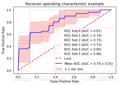
plt.plot(mean_fpr, mean_tpr, color='b',
         label=r'Mean ROC (AUC = %0.2f $\pm$ %0.2f)' % (mean_auc, std_auc),
         lw=2, alpha=.8)


std_tpr = np.std(tprs, axis=0)
tprs_upper = np.minimum(mean_tpr + std_tpr, 1)
tprs_lower = np.maximum(mean_tpr - std_tpr, 0)
plt.fill_between(mean_fpr, tprs_lower, tprs_upper, color='red', alpha=.2,
                 label=r'$\pm$ 1 std. dev.')

plt.xlim([-0.05, 1.05])
plt.ylim([-0.05, 1.05])
plt.xlabel('False Positive Rate')
plt.ylabel('True Positive Rate')
plt.title('Receiver operating characteristic example')
plt.legend(loc="lower right")
plt.show()

这里写图片描述

猜你喜欢