1、 计算图概念
1.1 Tensor
Tensor就是张量, 可以简单理解为多维数组,表明了数据结构
- 1
1.2 Flow
Flow 表达了张量之间通过计算相互转化的过程,体现了数据模型
- 1
1.3 数据流图基础
数据流图是每个 TensorFlow 程序的核心,用于定义计算结构

每一个节点都是一个运算,每一条边代表了计算之间的依赖关系
- 1
- 2
- 3
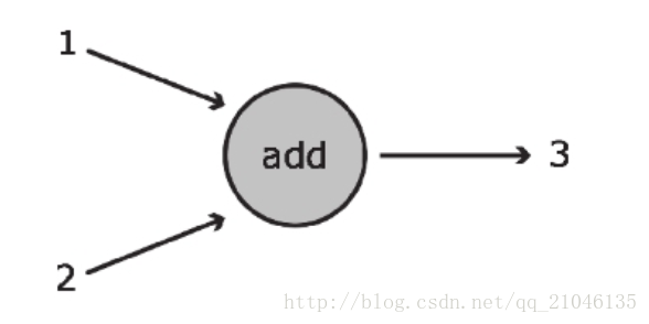
上图展示了可完成基本加法运算的数据流图。在该图中,加法运算是用圆圈表示的,它可接收两个输入 (以指向该函数的箭头表示),并将 1 和 2 之和 3 输出 (对应从该函数引出的箭头)。该函数的运算结果可传递给其他函数,也可直接返回给客户。
- 1
节点(node) :
在数据流图的语境中,节点通常以圆圈、椭圆和方框表示,代表了对数据所做的运算或某种操作。在上例中,“add”对应于一个孤立节点。
- 1
边(edge) :
对应于向Operation传入和从Operation传出的实际数值,通常以箭头表示。在“add”这个例子中,输入1和2均为指向运算节点的边,而输出3则为 从运算节点引出的边。可从概念上将边视为不同Operation之间的连接,因为它们将信息从一个节点传输到另一个节点。
- 1
2、计算图的使用
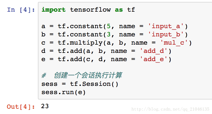
TensorFlow 程序一般可以分成两个阶段
    第一阶段 定义计算图中的所有计算
    第二阶段 为执行计算
- 1
- 2
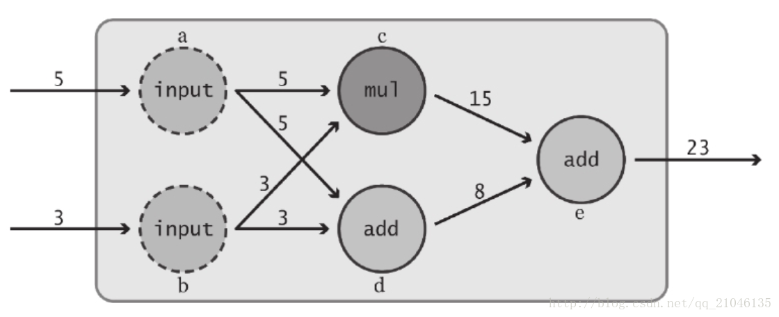
这里定义了 “input” 节点 a 和 b。语句第一次引用了 TensorFlow Operation:tf.constant()。在 TensorFlow 中,数据流图中的每个节点都被称为一个 Operation (简记为 Op )。各 Op 可接收 0 个或多个 Tensor 对象作为输入,并输出 0 个或多个 Tensor 对象。要创建一个 Op,可调用与其关联的 Python 构造方法,在本例中,tf.constant() 创建了一个 “常量” Op,它接收单个张量值,然后将同样的值输出给与其直接连接的节点。为方便起见,该函数自动将标量值 6 和 3 转换为 Tensor 对象。此外,我们还为这个构造方法传入了一个可选的字符串参数 name,用于对所创建的节点进行标识。
3、数据流图的可视化
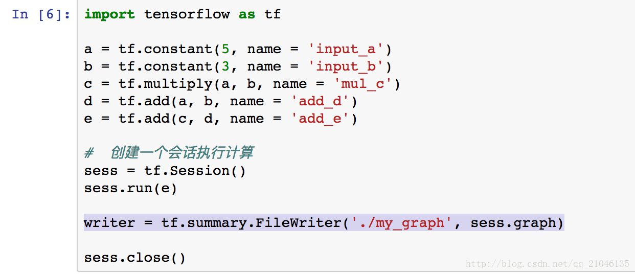
3.1 添加代码
writer = tf.summary.FileWriter('./my_graph', sess.graph)
- 1
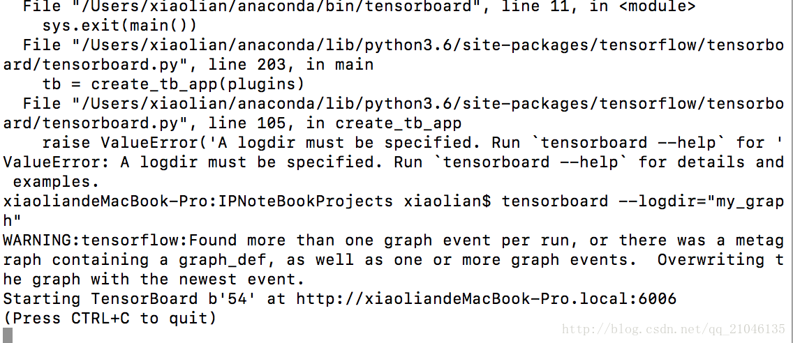
3.2 在 Terminal 输入命令
tensorboard --logdir="my_graph"
- 1
如图所示即成功
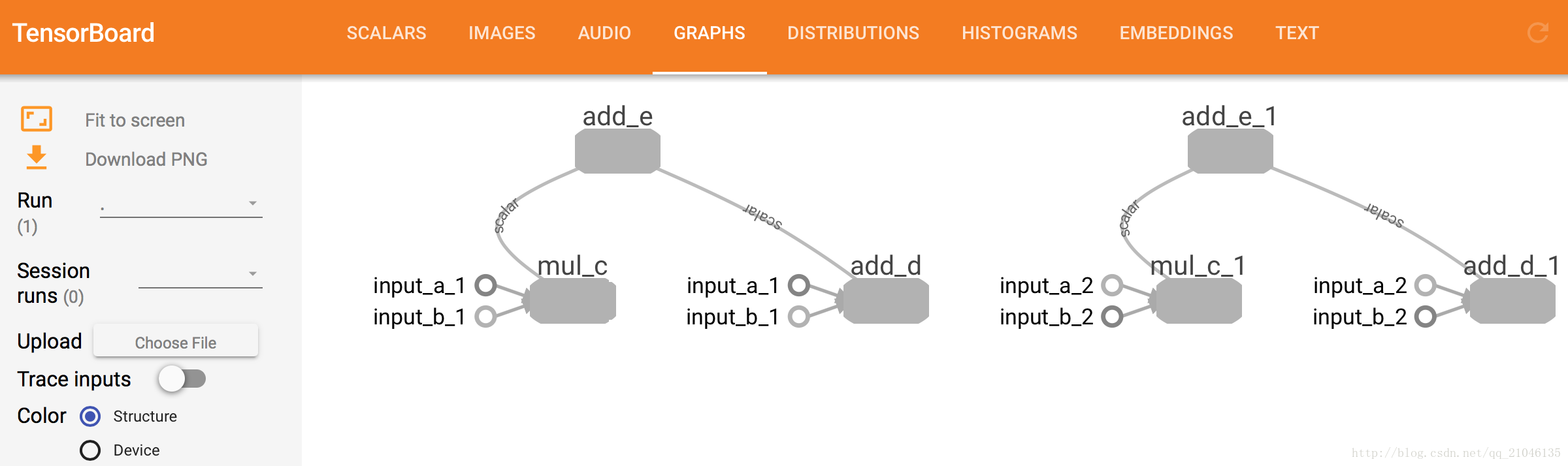
3.3 在浏览器输入 http://localhost:6006
切换到 GRAPHS 导航栏,就能看到数据流图
二、TnesorFlow 数据模型————张量
2.1 Python原生类型
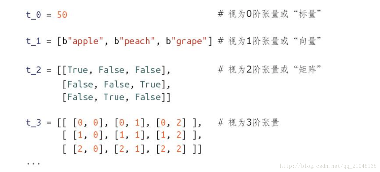
TensorFlow 可接收 Python 数值、布尔值、字符串或由它们构成的列表。单个数值将被转化为 0 阶张量(或标量),数值列表将被转化为 1 阶张量(向量),由列表构成的列表将被转化为 2 阶张量(矩阵),以此类推。下面给出一些例子。
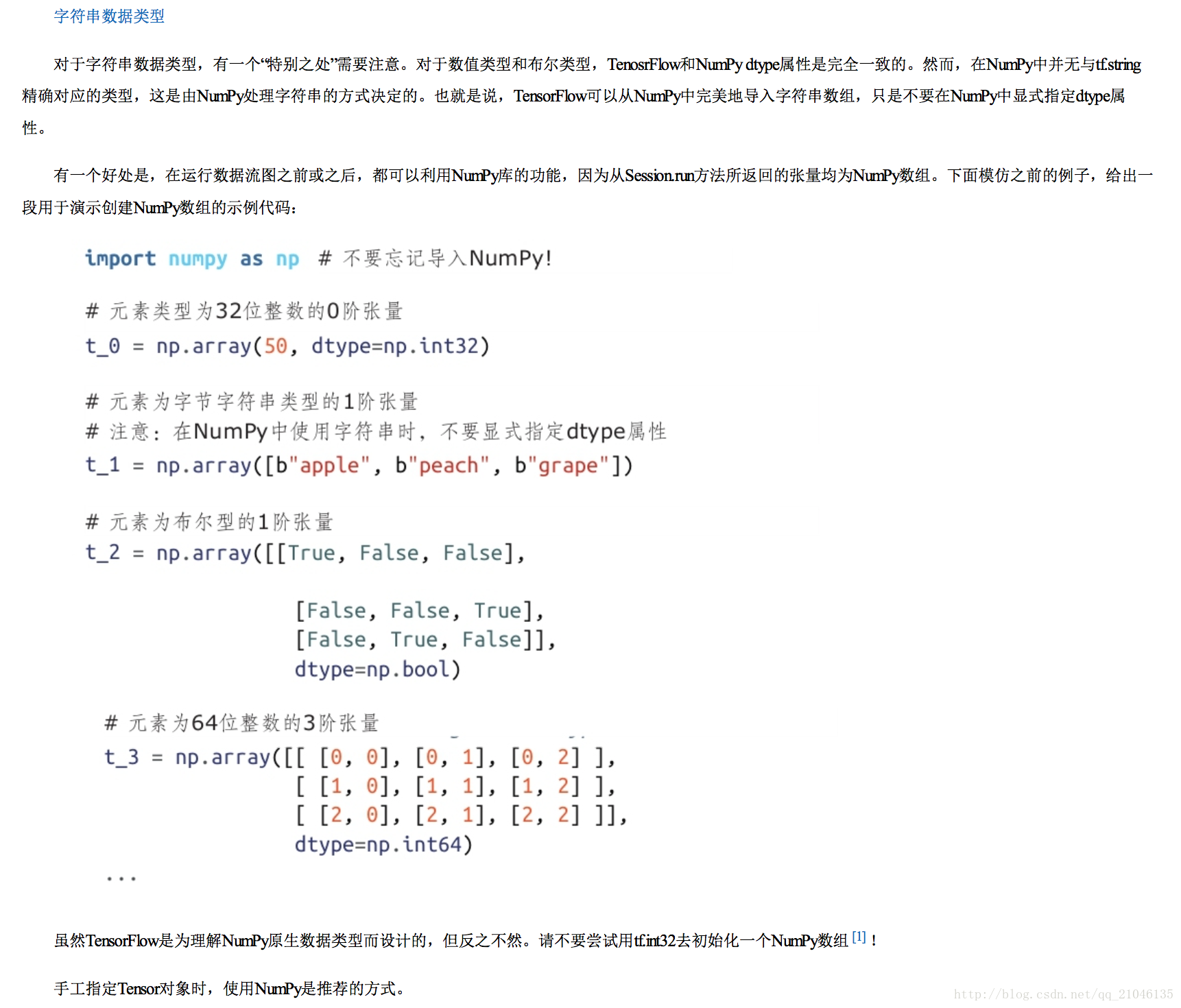
2.2 Numpy 类型
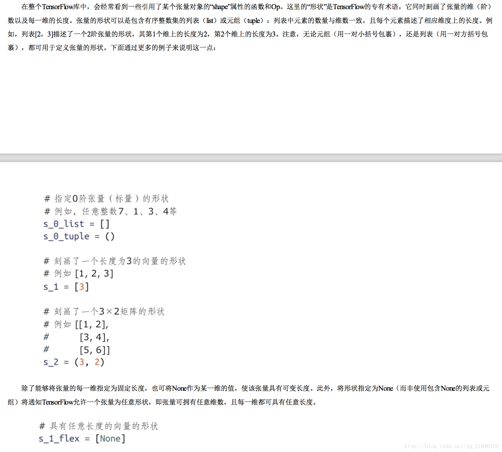
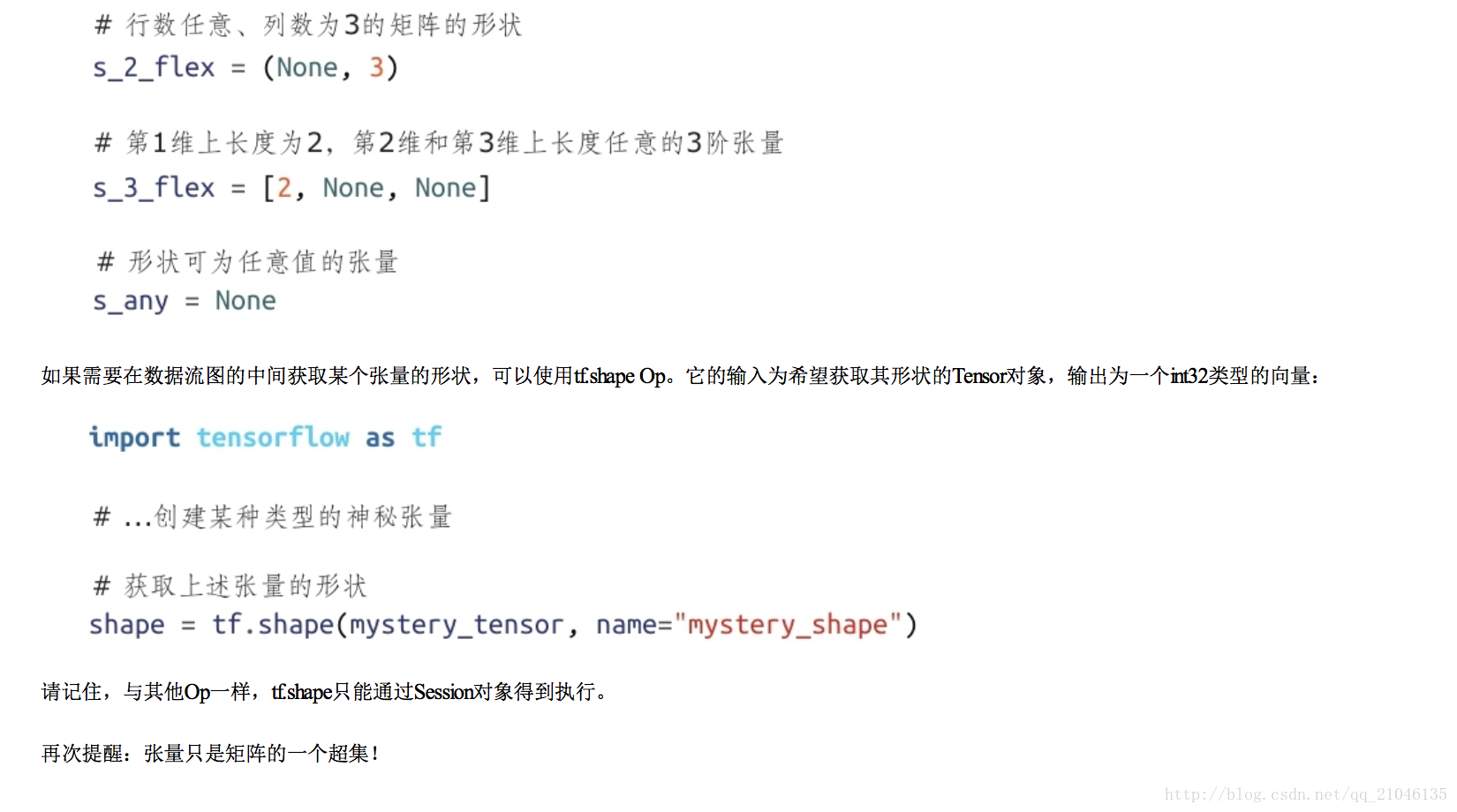
2.3 张量的形状
2.4 张量的使用
从上面的代码可以看出 TensorFlow 中的张量和 Numpy 中的数组不同,TensorFlow 计算的结果不是一个具体的数字, 而是一个张量的结构。
一个张量中主要保存了三个属性:名字(name),纬度(shape)和类型(type)。
名字(name):张量的第一个属性名字不仅是一个张量的唯一标识符,它同样也给出了这个张量是如何计算出来的
纬度(shape):描述了一个张量的维度信息
类型(type):每个张量会有一个唯一的类型
三、TnesorFlow 运行模型————会话
会话用来执行定义好的运算
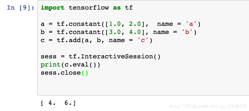
3.1 使用会话的模式一般有两种,第一种是需要明确调用会话生成函数和关闭会话函数
代码:
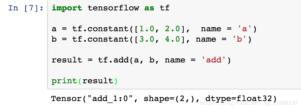
import tensorflow as tf

a = tf.constant([1.0, 2.0],  name = 'a')
b = tf.constant([3.0, 4.0],  name = 'b')
c = tf.add(a, b, name = 'c')

# 创建一个会话
sess = tf.Session()
sess.run(c)
# 关闭会话使得本次运行中使用到的资源可以被释放
sess.close()
- 1
- 2
- 3
- 4
- 5
- 6
- 7
- 8
- 9
- 10
- 11
- 12
然而,第一种模式在程序因异常退出时,关闭会话的函数可能不被执行从而导致资源泄漏, 第二种模式是通过上下文管理器来管理
import tensorflow as tf

a = tf.constant([1.0, 2.0],  name = 'a')
b = tf.constant([3.0, 4.0], name = 'b')
c = tf.add(a, b, name = 'c')

# 通过 python 中的上下文管理器来管理这个会话
with tf.Session() as sess:
    sess.run()

# 当上下文退出时会话关闭和资源释放也自动完成
- 1
- 2
- 3
- 4
- 5
- 6
- 7
- 8
- 9
- 10
- 11
3.2 交互式会话
在交互式环境下,通过设置默认会话的方式来获取张量的取值更加方便,使用 tf.InteractiveSession 会自动将生成的会话注册成为默认会话
四、利用占位节点添加输入
4.1 feed_dict 参数
参数 feed_dict 用于覆盖数据流图中的 Tensor 对象值,它需要 Python 字典对象作为输入。字典中的“键”为指向应当被覆盖的 Tensor 对象的句柄,而字典的“值”可以是 数字、字符串、列表或 NumPy 数组(之前介绍过)。这些“值”的类型必须与 Tensor 的“键”相同,或能够转换为相同的类型。下面通过一些代码来展示如何利用 feed_dict 重写之前的数据流图中a的值:
import tensorflow as tf

a = tf.add(2, 5)
b = tf.multiply(a, 3)

sess = tf.Session()

replace_dict = {a:15}

sess.run(b, feed_dict=replace_dict)
- 1
- 2
- 3
- 4
- 5
- 6
- 7
- 8
- 9
- 10
- 11
- 12
4.2 占位节点应用
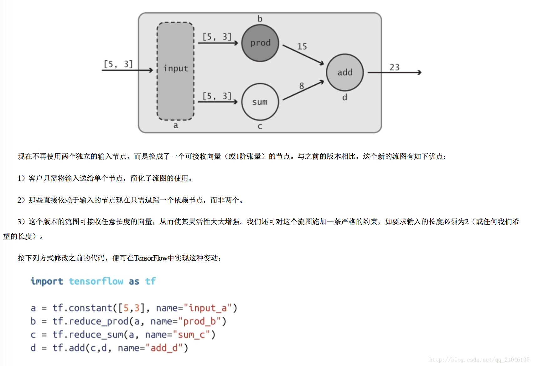
之前定义的数据流图并未使用真正的“输入”,它总是使用相同的数值 5 和 3。我们真正希望做的是从客户那里接收输入值,这样便可对数据流图中所描述的变换 以各种不同类型的数值进行复用,借助“占位符”可达到这个目的。正如其名称所预示的那样,占位符的行为与 Tensor 对象一致,但在创建时无须为它们指定具体的 数值。它们的作用是为运行时即将到来的某个 Tensor 对象预留位置,因此实际上变成了“输入”节点。利用 tf.placeholder Op 可创建占位符:
import tensorflow as tf
import numpy as np

a = tf.placeholder(tf.int32, shape=[2], name = 'my_input')
b = tf.reduce_prod(a, name = 'prod_a')
c = tf.reduce_sum(a, name = 'sum_c')

d = tf.add(b, c, name = 'add_d')

sess = tf.Session()

input_dict = {a : np.array([5, 3], dtype = np.int32)}

sess.run(d, feed_dict = input_dict)
- 1
- 2
- 3
- 4
- 5
- 6
- 7
- 8
- 9
- 10
- 11
- 12
- 13
- 14
- 15
输出:23
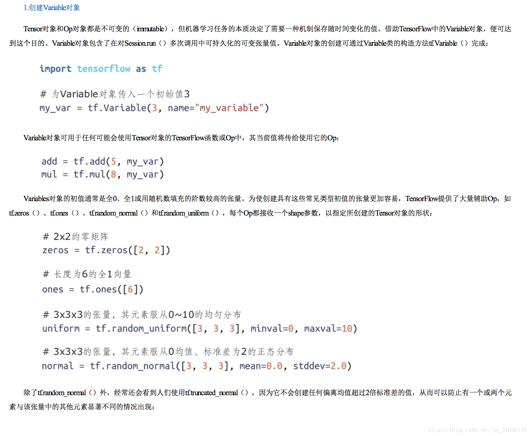
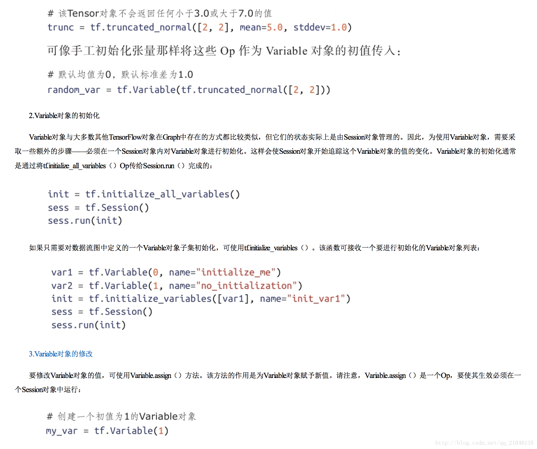
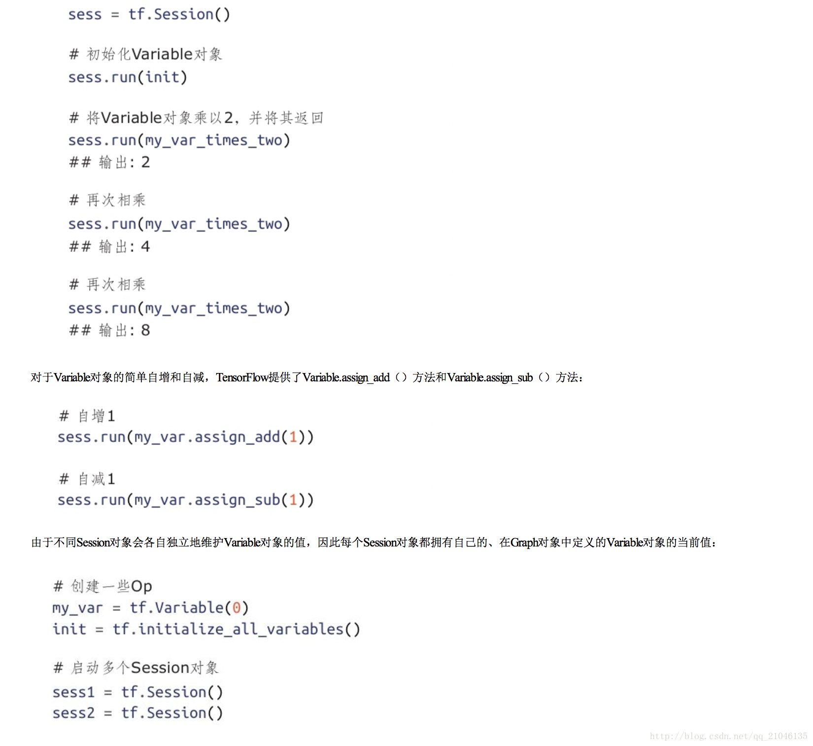
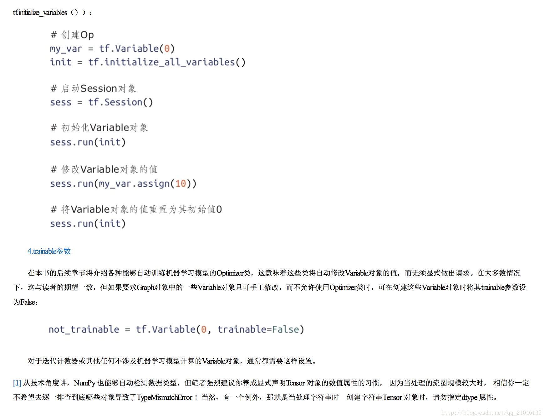
五、Variable 对象


六、名称作用域(name scope)
现实世界中的模型往往会包含几十或上百个节点,以及数以百万计的参数。为使这种级别的复杂性可控,TensorFlow当前提供了一种帮助用户组织数据流图的机制 ——名称作用域(name scope)。
程序1:
import tensorflow as tf

with tf.name_scope('scope_a'):
    a = tf.add(1,2, name = 'a')
    b = tf.multiply(3, 4, name = 'b')

with tf.name_scope('scope_b'):
    c = tf.add(4, 5, name = 'c')
    d = tf.multiply(6, 7, name = 'd')

writer = tf.summary.FileWriter('./name_scope_1', graph = tf.get_default_graph())
writer.close()
- 1
- 2
- 3
- 4
- 5
- 6
- 7
- 8
- 9
- 10
- 11
- 12

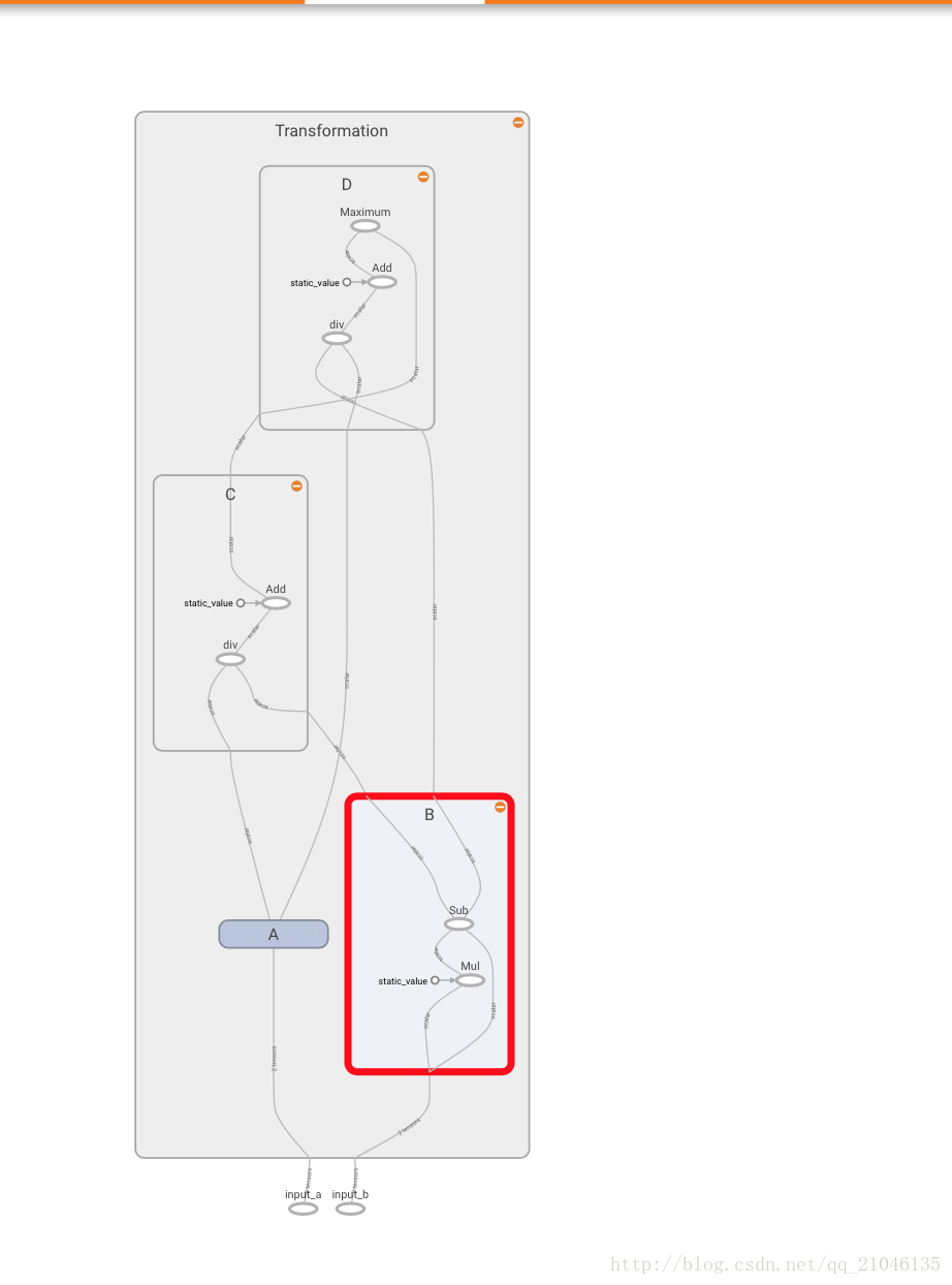
程序2:
import tensorflow as tf

graph = tf.Graph()

with graph.as_default():
    in_1 = tf.placeholder(tf.float32, shape = [], name = 'input_a')
    in_2 = tf.placeholder(tf.float32, shape = [], name = 'input_b')
    const = tf.constant(3, dtype = tf.float32, name = 'static_value')

    with tf.name_scope('Transformation'):

        with tf.name_scope('A'):
            A_mul = tf.multiply(in_1, const)
            A_out = tf.subtract(A_mul, in_1)

        with tf.name_scope('B'):
            B_mul = tf.multiply(in_2, const)
            B_out = tf.subtract(B_mul, in_2)

        with tf.name_scope('C'):
            C_div = tf.div(A_out, B_out)
            C_out = tf.add(C_div, const)

        with tf.name_scope('D'):
            D_div = tf.div(B_out, A_out)
            D_out = tf.add(D_div, const)
            out = tf.maximum(C_out, D_out)

        writer = tf.summary.FileWriter('./name_scope_2', graph = graph)
        writer.close()
- 1
- 2
- 3
- 4
- 5
- 6
- 7
- 8
- 9
- 10
- 11
- 12
- 13
- 14
- 15
- 16
- 17
- 18
- 19
- 20
- 21
- 22
- 23
- 24
- 25
- 26
- 27
- 28
- 29
- 30
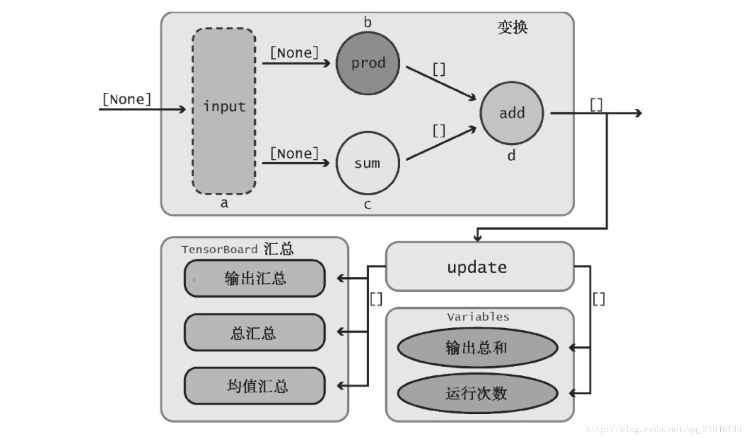
七、综合运用各种组件
7.1 数据流图
import tensorflow as tf

graph = tf.Graph()

with graph.as_default():

    with tf.name_scope("variables"):
        # 追踪数据流图运行次数
        global_step = tf.Variable(0, dtype = tf.int32, trainable = False, name = 'global_step')

        # 所有输出随时间的累加和
        total_output = tf.Variable(0.0, dtype = tf.float32, trainable = False, name = 'total_output')

    # 主要变换的 OP
    with tf.name_scope("transformation"):

        with tf.name_scope("input"):
            # 独立的输入层
            # 创建一个可以接收变量的占位符
            a = tf.placeholder(tf.float32, shape = [None], name = 'input_placeholder_a')

        # 独立的中间层
        with tf.name_scope("intermediate_layer"):
            b = tf.reduce_prod(a, name = 'b')
            c = tf.reduce_sum(a, name = 'c')

        # 独立的输出层
        with tf.name_scope("output"):
            output = tf.add(b, c, name = 'output')

    # 更新全局变量
    with tf.name_scope("update"):
        update_total = total_output.assign_add(output)
        increment_step = global_step.assign_add(1)

    #
    with tf.name_scope("summaries"):
        # 计算平均值
        avg = tf.div(update_total, tf.cast(increment_step, tf.float32), name = 'average')
        tf.summary.scalar('output', output)
        tf.summary.scalar('sum_of_outputs_overtime', update_total)
        tf.summary.scalar('average_of_outputs_over_time', avg)


    with tf.name_scope('global_ops'):
        # 初始化 OP
        init = tf.global_variables_initializer()
        # 将所有汇总数据合并到一个 OP 中
        merged_summaries = tf.summary.merge_all()


    sess = tf.Session(graph = graph)

    writer = tf.summary.FileWriter('./improved_graph', graph)

    sess.run(init)

    # 1)首先创建一个赋给Session.run()中feed_dict参数的字典,这对应于tf.placeholder节点,并用到了其句柄a。
    # 2)然后,通知Session对象使用feed_dict运行数据流图,我们希望确保output、increment_step以及merged_summaries Op能够得到执行。为写入汇总数据,需要保存 global_step和merged_summaries的值,因此将它们保存到Python变量step和summary中。这里用下划线“_”表示我们并不关心output值的存储。
    # 3)最后,将汇总数据添加到SummaryWriter对象中。global_step参数非常重要,因为它使TensorBoard可随时间对数据进行图示(稍后将看到,它本质上创建了一 个折线图的横轴)。
    def run_graph(input_tensor):
        feed_dict = {a : input_tensor}
        _, step, summary = sess.run([output, increment_step, merged_summaries], feed_dict = feed_dict)
        writer.add_summary(summary, global_step = step)


    run_graph([2, 8])
    run_graph([3, 1, 1, 3])

    writer.flush()
- 1
- 2
- 3
- 4
- 5
- 6
- 7
- 8
- 9
- 10
- 11
- 12
- 13
- 14
- 15
- 16
- 17
- 18
- 19
- 20
- 21
- 22
- 23
- 24
- 25
- 26
- 27
- 28
- 29
- 30
- 31
- 32
- 33
- 34
- 35
- 36
- 37
- 38
- 39
- 40
- 41
- 42
- 43
- 44
- 45
- 46
- 47
- 48
- 49
- 50
- 51
- 52
- 53
- 54
- 55
- 56
- 57
- 58
- 59
- 60
- 61
- 62
- 63
- 64
- 65
- 66
- 67
- 68
- 69
- 70
- 71
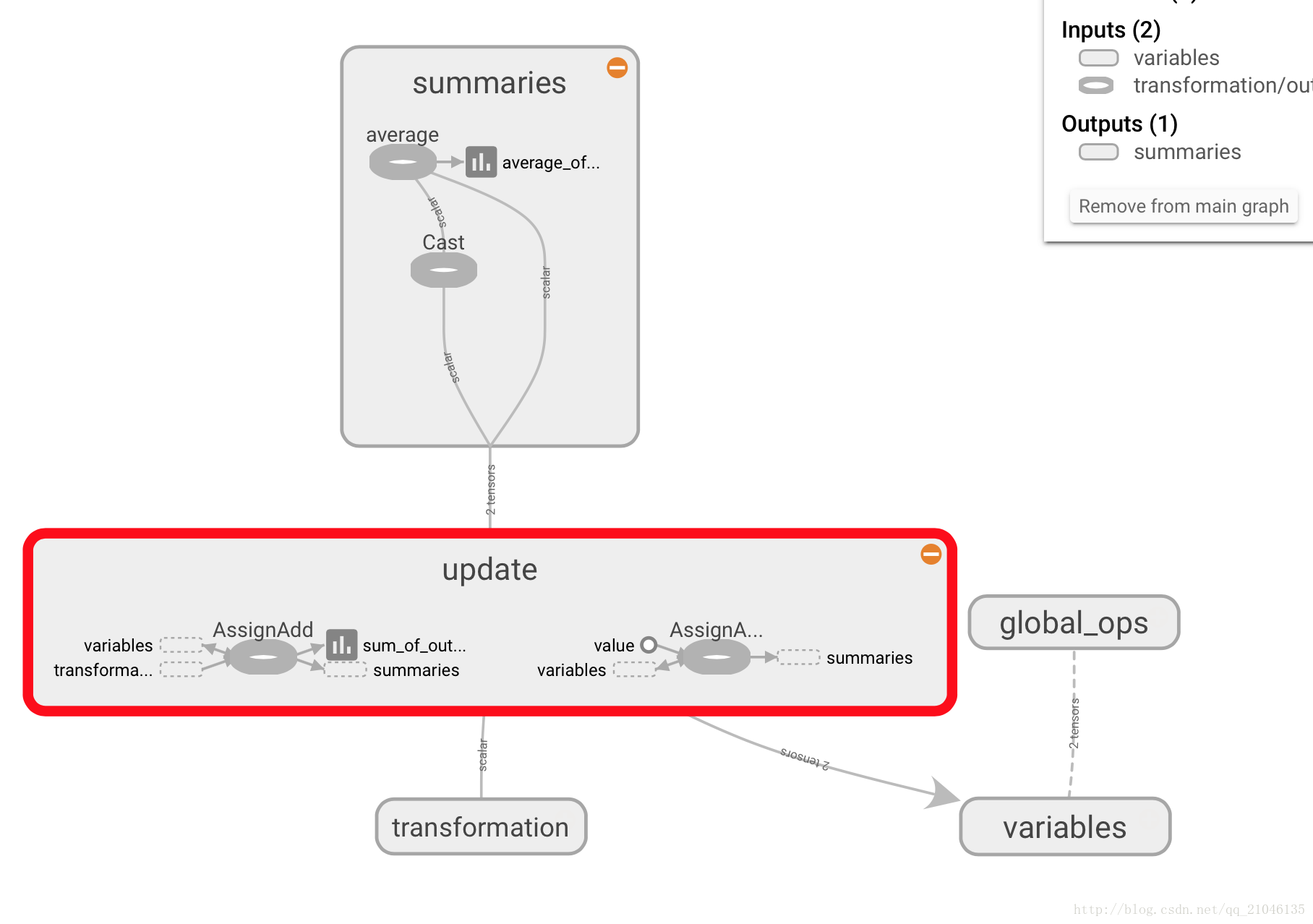
在 TensorBoard 显示为
八、TensorFlow 实现神经网络
8.1 神经网络解决分类问题主要步骤
1、提取问题中实体的特征向量作为神经网络的输入。不同的实体可以提取不同的特征向量
2、定义神经网络的结构,并定义如何从神经网络的输入得到输出,这个过程就是神经网络的前向传播算法
3、通过训练数据来调整神经网络中参数的取值
4、使用训练好的神经网络来预测未知的数据
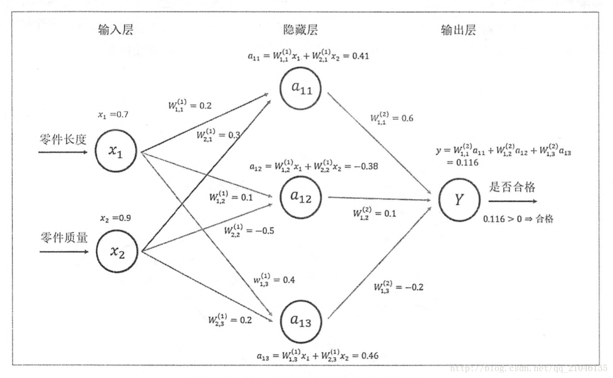
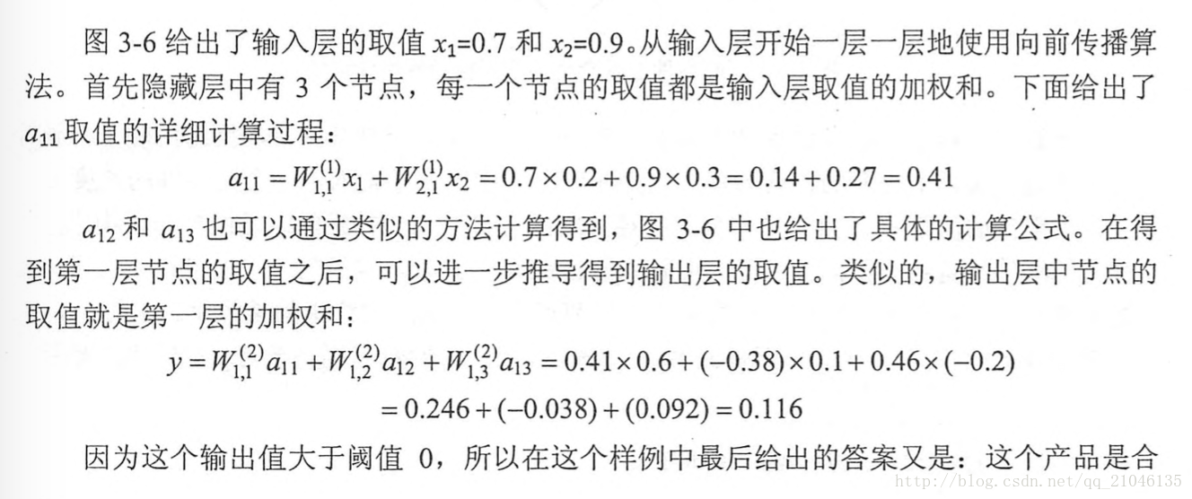
8.2 神经网络前向传播
示意图:
代码1:
import tensorflow as tf

w1 = tf.Variable(tf.random_normal([2, 3], stddev = 1, seed = 1))
w2 = tf.Variable(tf.random_normal([3, 1], stddev = 1, seed = 1))

x = tf.constant([[0.7, 0.9]])

a = tf.matmul(x, w1)
y = tf.matmul(a, w2)

sess = tf.Session()

sess.run(w1.initializer)
sess.run(w2.initializer)

print(sess.run(y))
sess.close()
- 1
- 2
- 3
- 4
- 5
- 6
- 7
- 8
- 9
- 10
- 11
- 12
- 13
- 14
- 15
- 16
- 17
代码2:使用占位函数,就不需要生成大量常量来提供输入数据
import tensorflow as tf

w1 = tf.Variable(tf.random_normal([2, 3], stddev = 1, seed = 1))
w2 = tf.Variable(tf.random_normal([3, 1], stddev = 1, seed = 1))

x = tf.placeholder(tf.float32, shape = (3, 2), name = 'input')

a = tf.matmul(x, w1)
y = tf.matmul(a, w2)

sess = tf.Session()
init = tf.initialize_all_variables()
sess.run(init)


print(sess.run(y, feed_dict = {x : [[0.7, 0.9], [0.1, 0.4], [0.5, 0.8]]}))
sess.close()
- 1
- 2
- 3
- 4
- 5
- 6
- 7
- 8
- 9
- 10
- 11
- 12
- 13
- 14
- 15
- 16
- 17
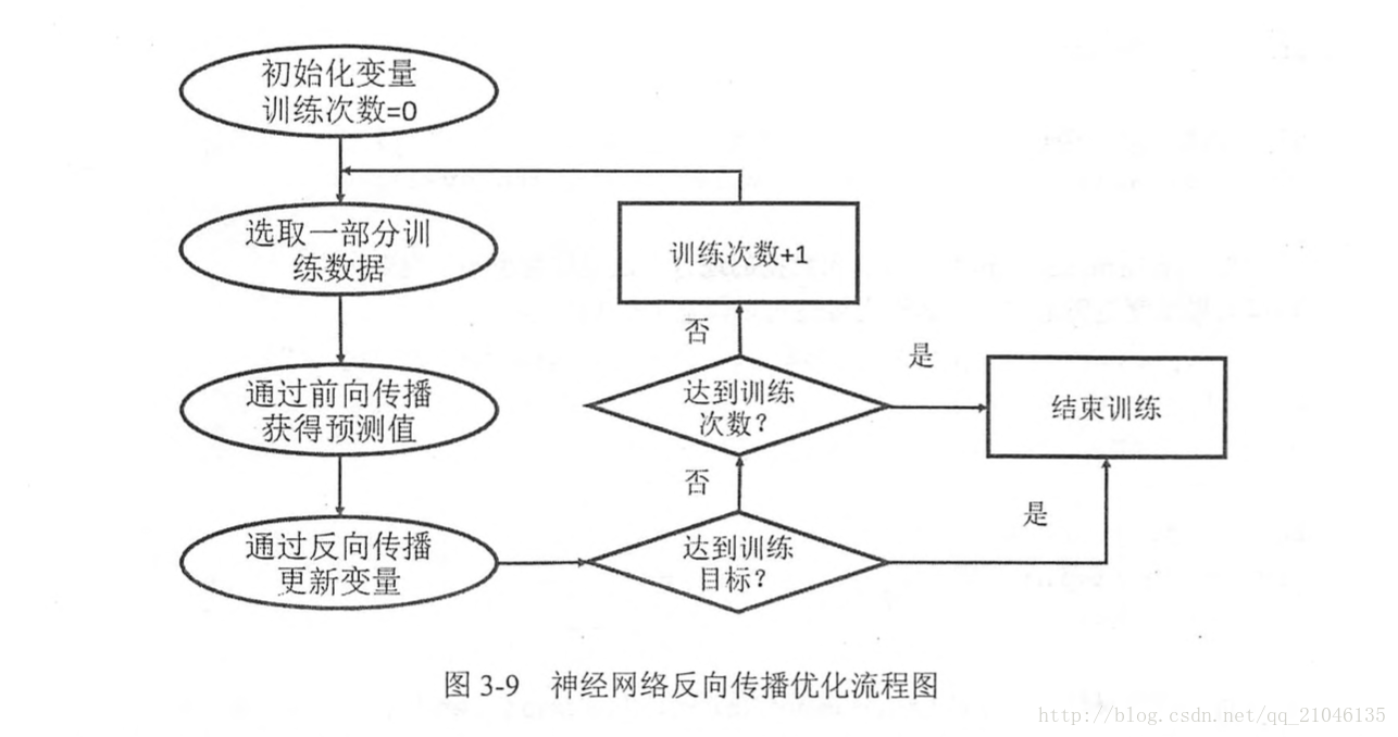
8.3 反向传播算法
在神经网络优化算法中,最常用的就是反向传播算法
8.4 神经网络完整程序
import tensorflow as tf
from numpy.random import RandomState

# 定义训练数据 batch 的大小
batch_size = 8

w1 = tf.Variable(tf.random_normal([2, 3], stddev = 1, seed = 1))
w2 = tf.Variable(tf.random_normal([3, 1], stddev = 1, seed = 1))

x = tf.placeholder(tf.float32 ,shape = (None, 2), name = 'x-input')
y_ = tf.placeholder(tf.float32, shape = (None, 1) ,name = 'y-input')

# 定义神经网络前向传播过程
a = tf.matmul(x, w1)
y = tf.matmul(a, w2)

# 定义损失函数和反向传播算法
cross_entropy = -tf.reduce_mean(y_ * tf.log(tf.clip_by_value(y, 1e-10, 1.0)))
train_step = tf.train.AdamOptimizer(0.001).minimize(cross_entropy)

# 通过随机数生成一个模拟数据集
rdm = RandomState(1)
dataset_size = 128
X = rdm.rand(dataset_size, 2)
Y = np.array([[int(x1 + x2 < 1) for (x1, x2) in X]]).reshape(128, 1)

with tf.Session() as sess:
    init = tf.initialize_all_variables()

    sess.run(init)

    print(sess.run(w1))
    print(sess.run(w2))

    # 设定训练轮数
    STEPS = 5000
    for i in range(STEPS):

        # 每次选取 batch_size 个样本进行训练
        start = (i * batch_size) % dataset_size
        end = min(start + batch_size, dataset_size)

        # 通过选取的样本训练神经网络并更新参数
        sess.run(train_step, feed_dict = {x : X[start : end], y_ : Y[start : end]})

        if i % 1000 == 0:
            # 每隔一段时间计算在所有数据上的交叉熵并输出
            total_cross_entropy = sess.run(cross_entropy, feed_dict = {x : X, y_ : Y})
            print("After %d training steps, cross entropy on all data is %g" % (i, total_cross_entropy))

    print(sess.run(w1))
    print(sess.run(w2))
- 1
- 2
- 3
- 4
- 5
- 6
- 7
- 8
- 9
- 10
- 11
- 12
- 13
- 14
- 15
- 16
- 17
- 18
- 19
- 20
- 21
- 22
- 23
- 24
- 25
- 26
- 27
- 28
- 29
- 30
- 31
- 32
- 33
- 34
- 35
- 36
- 37
- 38
- 39
- 40
- 41
- 42
- 43
- 44
- 45
- 46
- 47
- 48
- 49
- 50
- 51
- 52
输出:
[[-0.81131822  1.48459876  0.06532937]
 [-2.44270396  0.0992484   0.59122431]]
[[-0.81131822]
 [ 1.48459876]
 [ 0.06532937]]
After 0 training steps, cross entropy on all data is 0.0674925
After 1000 training steps, cross entropy on all data is 0.0163385
After 2000 training steps, cross entropy on all data is 0.00907547
After 3000 training steps, cross entropy on all data is 0.00714436
After 4000 training steps, cross entropy on all data is 0.00578471
[[-1.9618274   2.58235407  1.68203783]
 [-3.4681716   1.06982327  2.11788988]]
[[-1.8247149 ]
 [ 2.68546653]
 [ 1.41819501]]
- 1
- 2
- 3
- 4
- 5
- 6
- 7
- 8
- 9
- 10
- 11
- 12
- 13
- 14
- 15
					<link href="https://csdnimg.cn/release/phoenix/mdeditor/markdown_views-7b4cdcb592.css" rel="stylesheet">
            </div>