提取股票交易数据并对其进行分类

import sys
import numpy as np
import matplotlib
matplotlib.use(“TKAgg”)
import matplotlib.pyplot as plt
from matplotlib.collections import LineCollection

import pandas as pd

from sklearn import cluster,covariance,manifold

symbol_dict={‘TOT’: ‘Total’,
‘XOM’: ‘Exxon’,
‘CVX’: ‘Chevron’,
‘COP’: ‘ConocoPhillips’,
‘VLO’: ‘Valero Energy’,
‘MSFT’: ‘Microsoft’,
‘IBM’: ‘IBM’,
‘TWX’: ‘Time Warner’,
‘CMCSA’: ‘Comcast’,
‘CVC’: ‘Cablevision’,
‘YHOO’: ‘Yahoo’,
‘DELL’: ‘Dell’,
‘HPQ’: ‘HP’,
‘AMZN’: ‘Amazon’,
‘TM’: ‘Toyota’,
‘CAJ’: ‘Canon’,
‘SNE’: ‘Sony’,
‘F’: ‘Ford’,
‘HMC’: ‘Honda’,
‘NAV’: ‘Navistar’,
‘NOC’: ‘Northrop Grumman’,
‘BA’: ‘Boeing’,
‘KO’: ‘Coca Cola’,
‘MMM’: ‘3M’,
‘MCD’: ‘McDonald’s’,
‘PEP’: ‘Pepsi’,
‘K’: ‘Kellogg’,
‘UN’: ‘Unilever’,
‘MAR’: ‘Marriott’,
‘PG’: ‘Procter Gamble’,
‘CL’: ‘Colgate-Palmolive’,
‘GE’: ‘General Electrics’,
‘WFC’: ‘Wells Fargo’,
‘JPM’: ‘JPMorgan Chase’,
‘AIG’: ‘AIG’,
‘AXP’: ‘American express’,
‘BAC’: ‘Bank of America’,
‘GS’: ‘Goldman Sachs’,
‘AAPL’: ‘Apple’,
‘SAP’: ‘SAP’,
‘CSCO’: ‘Cisco’,
‘TXN’: ‘Texas Instruments’,
‘XRX’: ‘Xerox’,
‘WMT’: ‘Wal-Mart’,
‘HD’: ‘Home Depot’,
‘GSK’: ‘GlaxoSmithKline’,
‘PFE’: ‘Pfizer’,
‘SNY’: ‘Sanofi-Aventis’,
‘NVS’: ‘Novartis’,
‘KMB’: ‘Kimberly-Clark’,
‘R’: ‘Ryder’,
‘GD’: ‘General Dynamics’,
‘RTN’: ‘Raytheon’,
‘CVS’: ‘CVS’,
‘CAT’: ‘Caterpillar’,
‘DD’: ‘DuPont de Nemours’}

symbols,names=np.array(sorted(symbol_dict.items())).T
#sorted函数是必须的，要不然会报如下错误：iteration over a 0-d array，虽然有没有sorted函数，
#等号右边的格式都是<class ‘numpy.ndarray’>
#此前的理解是sorted只不过是按字母顺序排序的

quotes=[]
for symbol in symbols:
url=(“https://raw.githubusercontent.com/scikit-learn/examples-data/master/financial-data/{}.csv”)
quotes.append(pd.read_csv(url.format(symbol)))
#url.format(symbol)代表的是不同symbols对应的URL，URL中的{}将被不同的symbol替换。
#通过pd.read_csv读取相应的数据，存入quotes中。所以quotes将会有len(symbols)=56个存储单元
#每个存储单元里包含datetime,open,close对应的数值，本例中每个单元中包含1258条数据。

close_prices=np.vstack([q[“close”] for q in quotes]) #shape is 561258
open_prices=np.vstack([q[“open”] for q in quotes])#shape is 561258

variation = close_prices - open_prices #close和open中的对应数值做相应运算shape is 56*1257
print(variation.shape)

Learn a graphical structure from the correlations

edge_model = covariance.GraphicalLassoCV(cv=5)

standardize the time series: using correlations rather than covariance

is more efficient for structure recovery

X = variation.copy().T #changed the shape,which now is 125856,1258 samples,56 features
X /= X.std(axis=0) #除以本列的标准查
edge_model.fit(X) #通过拟合，可以返回5656的协方差，用来反应不同的stock和stock之间的线性关系

Cluster using affinity propagation

, labels = cluster.affinity_propagation(edge_model.covariance)#根据协方差进行聚类分析
n_labels = labels.max() #类的个数为labels.max() +1

for i in range(n_labels + 1):
print(‘Cluster %i: %s’ % ((i + 1), ', '.join(names[labels == i])))
#names和labels位置是一致的，一一对应的，不同位置在labels中的值一致的话，则归为一类

Find a low-dimension embedding for visualization: find the best position of

the nodes (the stocks) on a 2D plane

We use a dense eigen_solver to achieve reproducibility (arpack is

initiated with random vectors that we don’t control). In addition, we

use a large number of neighbors to capture the large-scale structure.

node_position_model = manifold.LocallyLinearEmbedding(
n_components=2, eigen_solver=‘dense’, n_neighbors=6)

embedding = node_position_model.fit_transform(X.T).T #X.T的降纬处理，处理后为2纬

Visualization

plt.figure(1, facecolor=‘w’, figsize=(10, 8))
plt.clf()
ax = plt.axes([0., 0., 1., 1.])
plt.axis(‘off’)

Display a graph of the partial correlations

partial_correlations = edge_model.precision_.copy()
d = 1 / np.sqrt(np.diag(partial_correlations))
partial_correlations *= d
partial_correlations *= d[:, np.newaxis]
non_zero = (np.abs(np.triu(partial_correlations, k=1)) > 0.02) #np.triu返回上角矩阵

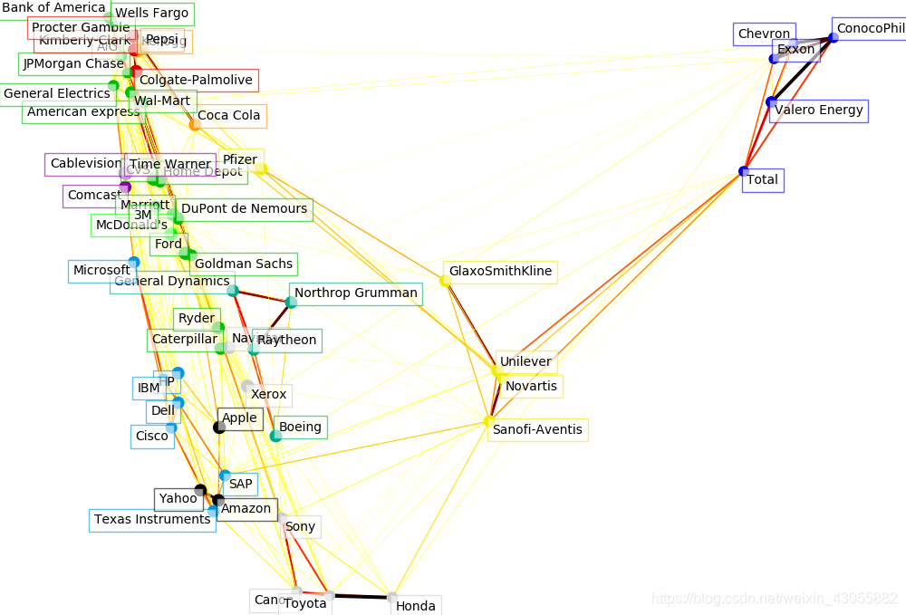
Plot the nodes using the coordinates of our embedding

#x=embedding[0],y=embedding[1],画出代表股票的点
plt.scatter(embedding[0], embedding[1], s=100 * d ** 2, c=labels,
cmap=plt.cm.nipy_spectral)

Plot the edges，画出股票之间的连线，粗细(values)表示两者之间的相关性

start_idx, end_idx = np.where(non_zero)#以元组形式返回值为true的坐标

a sequence of (line0, line1, line2), where::

linen = (x0, y0), (x1, y1), … (xm, ym)

segments = [[embedding[:, start], embedding[:, stop]]
for start, stop in zip(start_idx, end_idx)]
values = np.abs(partial_correlations[non_zero]) #行列式子变换后的矩阵的非零值
lc = LineCollection(segments,
zorder=0, cmap=plt.cm.hot_r,
norm=plt.Normalize(0, .7 * values.max()))
lc.set_array(values)
lc.set_linewidths(10 * values)
ax.add_collection(lc)

Add a label to each node. The challenge here is that we want to

position the labels to avoid overlap with other labels

#x,y为表示股票坐标的点的坐标
for index, (name, label, (x, y)) in enumerate(
zip(names, labels, embedding.T)):

dx = x - embedding[0] #某一个点的横坐标于其他所有点的横坐标的差值，长度为56
dx[index] = 1 #设第index个值为1，原值为0
dy = y - embedding[1]#某一个点的纵坐标于其他所有点的纵坐标的差值，长度为56
dy[index] = 1#设第index个值为1，原值为0
this_dx = dx[np.argmin(np.abs(dy))]
#np.argmin()返回最小值所在的下标,本语句为求出dy绝对值最小值所在的dx坐标
this_dy = dy[np.argmin(np.abs(dx))]
#np.argmin()返回最小值所在的下标,本语句为求出dy绝对值最小值所在的dx坐标
if this_dx > 0:
    horizontalalignment = 'left'
    x = x + .002
else:
    horizontalalignment = 'right' 
    x = x - .002
if this_dy > 0:
    verticalalignment = 'bottom'
    y = y + .002
else:
    verticalalignment = 'top'
    y = y - .002
plt.text(x, y, name, size=10,
         horizontalalignment=horizontalalignment,
         verticalalignment=verticalalignment,
         bbox=dict(facecolor='w',
                   edgecolor=plt.cm.nipy_spectral(label / float(n_labels)),
                   alpha=.6))

plt.xlim(embedding[0].min() - .15 * embedding[0].ptp(),
embedding[0].max() + .10 * embedding[0].ptp(),)
plt.ylim(embedding[1].min() - .03 * embedding[1].ptp(),
embedding[1].max() + .03 * embedding[1].ptp())

plt.show()

PS：来自sklearn的教学案例，加了一下解释，方便自己以后看的时候轻松点。自己做的分类像个屎，就不放了