Table of Contents
PCA对比理解与实现
一、numpy方式
1.数据基本导入
from sklearn.datasets import load_iris
import matplotlib.pyplot as plt
%matplotlib inline
iris = load_iris()
iris_X, iris_y = iris.data, iris.target
iris_X[0:10]
array([[ 5.1,  3.5,  1.4,  0.2],
       [ 4.9,  3. ,  1.4,  0.2],
       [ 4.7,  3.2,  1.3,  0.2],
       [ 4.6,  3.1,  1.5,  0.2],
       [ 5. ,  3.6,  1.4,  0.2],
       [ 5.4,  3.9,  1.7,  0.4],
       [ 4.6,  3.4,  1.4,  0.3],
       [ 5. ,  3.4,  1.5,  0.2],
       [ 4.4,  2.9,  1.4,  0.2],
       [ 4.9,  3.1,  1.5,  0.1]])
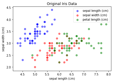
2. 绘图函数定义
label_dict = {i:k for i,k in enumerate(iris.feature_names)}

def plot(X, y, title, x_label, y_label):
    ax = plt.subplot(111)
    for label, marker, color in zip(range(3), ('^', 's', '0'), ('blue','red','green')):
        plt.scatter(x=X[:, 0].real[y==label],y=X[:,1].real[y==label],color=color,alpha=0.5,label=label_dict[label])
        plt.xlabel(x_label)
        plt.ylabel(y_label)
        leg = plt.legend(loc='upper right', fancybox=True)
        leg.get_frame().set_alpha(0.5)
        plt.title(title)
plot(iris_X, iris_y, "original iris data", "sepal length (cm)", "sepal width(cm)")

4.计算pca
协方差矩阵
import numpy as np
mean_vector = iris_X.mean(axis=0)
cov_mat = np.cov((iris_X-mean_vector).T)
协方差矩阵的特征值求解
eig_val_cov, eig_vec_cov = np.linalg.eig(cov_mat)
for i in range(len(eig_val_cov)):
    eigvec_cov = eig_vec_cov[:,i]
    print('eigenvector {}: \n{}'.format(i+1, eigvec_cov))
    print('eigenvalue {} from covariance matrix: {}'.format(i+1, eig_val_cov[i]))
    print(30 * '-')
eigenvector 1:
[ 0.36158968 -0.08226889  0.85657211  0.35884393]
eigenvalue 1 from covariance matrix: 4.22484076832011
------------------------------
eigenvector 2:
[-0.65653988 -0.72971237  0.1757674   0.07470647]
eigenvalue 2 from covariance matrix: 0.2422435716275147
------------------------------
eigenvector 3:
[-0.58099728  0.59641809  0.07252408  0.54906091]
eigenvalue 3 from covariance matrix: 0.07852390809415469
------------------------------
eigenvector 4:
[ 0.31725455 -0.32409435 -0.47971899  0.75112056]
eigenvalue 4 from covariance matrix: 0.023683027126001316
------------------------------
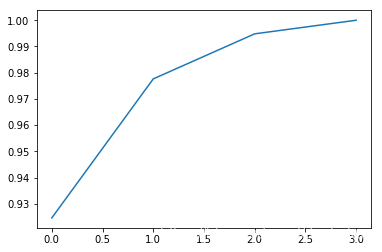
查看几个特征值的重要性
explained_variance_ratio = eig_val_cov/eig_val_cov.sum()
print(explained_variance_ratio)
plt.plot(np.cumsum(explained_variance_ratio))
[ 0.92461621  0.05301557  0.01718514  0.00518309]


[<matplotlib.lines.Line2D at 0x93f2550>]
5.应用求得到的特征值对原数据集进行转换
top_2_eigenvectors = eig_vec_cov[:,:2].T
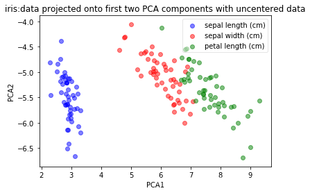
1.未进行中心化
np.dot(iris_X, top_2_eigenvectors.T)[:5, ]
array([[ 2.82713597, -5.64133105],
       [ 2.79595248, -5.14516688],
       [ 2.62152356, -5.17737812],
       [ 2.7649059 , -5.00359942],
       [ 2.78275012, -5.64864829]])
plot(np.dot(iris_X, top_2_eigenvectors.T), iris_y, 'iris:data projected onto first two PCA components with uncentered data', 'PCA1','PCA2')
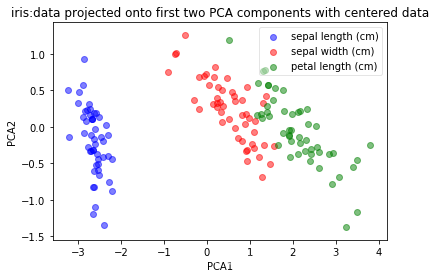
2.进行中心化之后
np.dot(iris_X-mean_vector, top_2_eigenvectors.T)[:5, ]
array([[-2.68420713, -0.32660731],
       [-2.71539062,  0.16955685],
       [-2.88981954,  0.13734561],
       [-2.7464372 ,  0.31112432],
       [-2.72859298, -0.33392456]])
plot(np.dot(iris_X-mean_vector, top_2_eigenvectors.T), iris_y, 'iris:data projected onto first two PCA components with centered data', 'PCA1','PCA2')
二、采用sklearn
from sklearn.decomposition import PCA
pca = PCA(n_components=2)
1.拟合与训练
pca.fit(iris_X)
PCA(copy=True, iterated_power='auto', n_components=2, random_state=None,
  svd_solver='auto', tol=0.0, whiten=False)
2.top2的特征值结果
pca.components_
array([[ 0.36158968, -0.08226889,  0.85657211,  0.35884393],
       [ 0.65653988,  0.72971237, -0.1757674 , -0.07470647]])
pca.transform(iris_X)[:5,]
array([[-2.68420713,  0.32660731],
       [-2.71539062, -0.16955685],
       [-2.88981954, -0.13734561],
       [-2.7464372 , -0.31112432],
       [-2.72859298,  0.33392456]])
这里的结果与采用numpy上面的1结果不相同,原因:sklearn中对irri_X进行转换之前,已经进行中心化.
1、中心化的好处?
plot(iris_X, iris_y, "Original Iris Data", "sepal length (cm)", "sepal width (cm)")
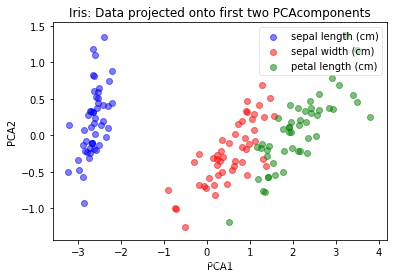
plot(pca.transform(iris_X), iris_y, "Iris: Data projected onto first two PCAcomponents", "PCA1", "PCA2")
3.特征值的重要性(对原数据的可解释性)
pca.explained_variance_ratio_
array([ 0.92461621, 0.05301557])
三、PCA对特征非相关的处理
np.corrcoef(iris_X.T)
array([[ 1.        , -0.10936925,  0.87175416,  0.81795363],
       [-0.10936925,  1.        , -0.4205161 , -0.35654409],
       [ 0.87175416, -0.4205161 ,  1.        ,  0.9627571 ],
       [ 0.81795363, -0.35654409,  0.9627571 ,  1.        ]])
np.corrcoef(iris_X.T)[[0,0,0,1,1],[1,2,3,2,3]]
array([-0.10936925, 0.87175416, 0.81795363, -0.4205161 , -0.35654409])
np.corrcoef(iris_X.T)[[0,0,0,1,1],[1,2,3,2,3]].mean()
0.1606556709416852
上面的结果看到,变量之间的相关系数平均值0.16>0
full_pca = PCA(n_components=4)
full_pca.fit(iris_X)
PCA(copy=True, iterated_power='auto', n_components=4, random_state=None,
  svd_solver='auto', tol=0.0, whiten=False)
full_pca
PCA(copy=True, iterated_power='auto', n_components=4, random_state=None,
  svd_solver='auto', tol=0.0, whiten=False)
#
pac_iris = full_pca.transform(iris_X)
np.corrcoef(pac_iris.T)[[0,0,0,1,1],[1,2,3,2,3]].mean()
-2.9630768059673058e-16
从上面结果看,新的变量的相关关系平均系数约为0
结论:PCA助于减缓特征变量之间的相关性,即使是不减少变量数量
四、 关于center和standardization的作用
函数的简单说明:
- StandardScaler(with_mean,with_std)
- 功能:实现对数据转换成标准正态分布.
- 参数:with_mean=True(default)表示均值归一化到0;with_std=True(default)表示标准差归一化到1.
from sklearn.preprocessing import StandardScaler
1.采用非标准整体分布形式
X_centered = StandardScaler(with_std=False).fit_transform(iris_X)
X_centered[:5,]
array([[-0.74333333,  0.446     , -2.35866667, -0.99866667],
       [-0.94333333, -0.054     , -2.35866667, -0.99866667],
       [-1.14333333,  0.146     , -2.45866667, -0.99866667],
       [-1.24333333,  0.046     , -2.25866667, -0.99866667],
       [-0.84333333,  0.546     , -2.35866667, -0.99866667]])
iris_X[:5,]
array([[ 5.1,  3.5,  1.4,  0.2],
       [ 4.9,  3. ,  1.4,  0.2],
       [ 4.7,  3.2,  1.3,  0.2],
       [ 4.6,  3.1,  1.5,  0.2],
       [ 5. ,  3.6,  1.4,  0.2]])
X_centered.std(axis=0)
array([ 0.82530129, 0.43214658, 1.75852918, 0.76061262])
plot(X_centered, iris_y, 'iris_data centered', 'sepal lenght(cm)','sepal_width(cm)')
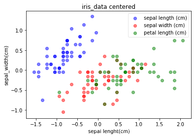
从分布上看,与未centerd的数据无区别。
pca.fit(X_centered)
PCA(copy=True, iterated_power='auto', n_components=2, random_state=None,
  svd_solver='auto', tol=0.0, whiten=False)
pca.components_
array([[ 0.36158968, -0.08226889,  0.85657211,  0.35884393],
       [ 0.65653988,  0.72971237, -0.1757674 , -0.07470647]])
pca.transform(X_centered)[:5,]
array([[-2.68420713,  0.32660731],
       [-2.71539062, -0.16955685],
       [-2.88981954, -0.13734561],
       [-2.7464372 , -0.31112432],
       [-2.72859298,  0.33392456]])
plot(pca.transform(X_centered), iris_y, 'iris:data projected onto first two PCA components with centered data', 'PCA1','PCA2')
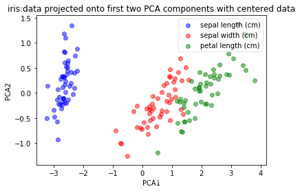
- 从经过centered的结果上看,在PCA结果分布上面无区别。
- 原因:因为在center前后,两份数据的协方差相同,因此特征分解结果相同
2.采用标准正态分布的形式
X_scaled = StandardScaler().fit_transform(iris_X)
plot(X_scaled, iris_y, 'iris:data scaled', 'sepal length(cm)', 'sepal width(cm)')

pca.fit(X_scaled)
PCA(copy=True, iterated_power='auto', n_components=2, random_state=None,
  svd_solver='auto', tol=0.0, whiten=False)
pca.components_
array([[ 0.52237162, -0.26335492,  0.58125401,  0.56561105],
       [ 0.37231836,  0.92555649,  0.02109478,  0.06541577]])
从上面的主成分结果看,已经发生变化。当我们scaling时候,意味着center和除标准差.
pca.transform(X_scaled)[:5,]
array([[-2.26454173,  0.5057039 ],
       [-2.0864255 , -0.65540473],
       [-2.36795045, -0.31847731],
       [-2.30419716, -0.57536771],
       [-2.38877749,  0.6747674 ]])
pca.explained_variance_ratio_
array([ 0.72770452, 0.23030523])
主成分可解释性有变化
plot(pca.transform(X_scaled), iris_y, 'iris:data projected onto first two PCA components', 'PCA1','PCA2')
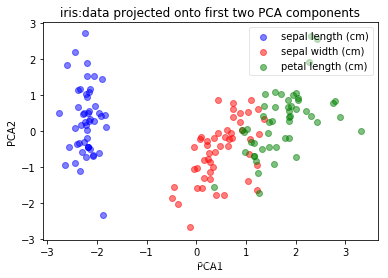
结论:center和scaling不改变数据的shape,但影响feature interaction
参考自:
(1)Sinan Ozdemir, Divya Susarla的一本书