Acceleration Structures

Acceleration Structures

ray-tracing, bounding box, grid, BVH, space partitioning data structure, k-d tree, octree, spatial division, spatial coherence, space tracing, 3D-Digital Differential Analyser, DDA

1. Introduction

以Utah Teapot茶壶为例，在三角面片与场景中的绘制对象数量增多时，ray-tracing会变得很慢，它最花时间的步骤是intersection test求交步骤，因为对画面的每个pixel我们都需要去对每个三角面片进行求交测试。

Accelerated Ray Tracing" (1983), Fujimoto: The calculation speed of the ray-tracing method is undoubtedly one of the basic problems that must be dealt with. Why is raytracing so computationally expensive? The main cause was clearly identified at the very moment ray tracing first entered the field of computer graphics. According to Whitted, for simple scenes 75 percent of the total time is spent on calculating intersections between rays and objects. For more complex scenes the proportion goes as high as 95 percent. The time that must be spent calculating the intersections is directly related to the number of objects involved in the-scene".

因此为了节省渲染所需时间，我们需要尽可能的减少求交测试的数量。Acceleration Structure的核心思想是以最快的速度去决定场景中哪些物体会与特定的光线相交，并以此来避免计算那些不必要进行求交的测试。理论上来说，使用这种Structure可以降低需要进行求交测试物体数量的50%，也就是可以从理论上减少渲染所需时间的50%

2. Bounding Volume —— Bounding Box

Bounding Box理论上来说不能算是一种Acceleration Structure，但是这确实是最简单的一种降低渲染时间的方法。对于茶壶的每个网格而言，都有可能存在超过100个需要绘制的三角面片，即需要相应数量的求交测试去进行场景的渲染。Bounding Box所做的事情，是是用一些盒子去包围茶壶的网格，然后用这些盒子代替对网格进行ray-trace。

bounding volume: it is the tightest possible volume (a box in that case but it could also be a sphere) surrounding the grid. Figure 1 shows the bounding boxes of each one of the 32 Bézier patches making up the teapot model.

我们首先对这些Bounding Box进行求交，如果发现光线与这些盒子都没有相交，name就可以直接排除掉这些内容，不需要进行下一步的求交测试，如下图的内容所示，如果只有绿色部分的Bounding Box被红色的指定光线穿过，而其他的Box与该光线没有相交，那么可以直接排除掉除了绿色Box以外的内容，只对绿色Box内的三角面片进行求交测试。由于和指定光线方向追踪想交Bounding Box占总Bounding Box的数量一般来说是比较小的，所以进行这些操作可以节省很大一部分的渲染时间。

for object in scene:
  if intersect(ray, boundingBox(object)):
    for triangle in object:
      if intersect(ray, triangle):
        // ray intersects operation
        ... 

计算Object的Bounding Box是非常简单的，我们只要遍历这个物体的所有顶点坐标，分别取出xyz的最大值和最小值，作为Bounding Box的两个顶点即可，如下图所示：

3. Bounding Volume Hierarchy

Ray Tracing Complex Scenes, Kay and Kajiya, 1986

上文的Bounding Box的ray-tracing方法确实可以直观的表现出如何可以快速的降低渲染所需时间，但是Bounding Box也有它的缺陷，在Bounding Box的边界过于宽松的时候，这个方法就显得比较冗余，以下图为例，两条黄色的光线是显然不会与茶壶相交的，但是如果使用简单的Bounding Box，它们会被进行求交计算，这些操作是多余的。

Figure 1: when the bounding voume representing an object fits the object too loosely, many rays intersecting the extent do not intersect with the shape and are wasted (top). Using a more complex bounding volume (bottom) gives better results but is more costly to ray trace.

一方面，虽然Bounding Box或者是Bounding Sphere等一些最简单的几何体可以解决绝大部分的性能问题，另一方面最完美的Bounding Volume其实是绘制对象本身的几何，但这样又回到了最原始的ray-tracing问题。那么，如何在对Object的紧贴程度和计算速度之间找到最优的Bounding Volume的成为了现在最重要的问题。

A good choice for a bounding volume is therefore a shape that provides a good tradeoff between tightness (how close an extent fits the object) and speed (a complex bounding volume is more expensive to ray trace than a simple shape).

Kay和Kajiya在1986年的文章剔除一些对于Bounding Volume算法的核心思想，一个Bounding Box可以看成几个相交的平面，分开xyz三个方向可以看做是每个维度中，使用两个平行的平面去夹住分析的几何对象，类似下图：

这样就做出了上一节中所使用的最简单的Bounding Box，这个盒子的边都平行于xyz坐标轴，name更进一步，如果不只是使用三对平行的平面去夹住对象几何体呢，比如下图所示的2D空间下的例子：

对于3D空间，Kay和Kajiya使用了7对对平面坐标，即一个和xyz轴平行的Bounding Box与一个八面体结构包围的Bounding Volume：
$\begin{array}{l} {\left(\begin{array}{c} 1\\0\\0 \end{array}\right),\; \left(\begin{array}{c} 0\\1\\0 \end{array}\right),\; \left(\begin{array}{c}0\\0\\1 \end{array}\right), } { \left(\begin{array}{c} \dfrac{\sqrt{3}}{3}\\ \dfrac{\sqrt{3}}{3}\\ \dfrac{\sqrt{3}}{3} \end{array}\right),\; \left(\begin{array}{c} -\dfrac{\sqrt{3}}{3}\\ \dfrac{\sqrt{3}}{3}\\ \dfrac{\sqrt{3}}{3} \end{array}\right),\; \left(\begin{array}{c} -\dfrac{\sqrt{3}}{3}\\ -\dfrac{\sqrt{3}}{3}\\ \dfrac{\sqrt{3}}{3} \end{array}\right), \left(\begin{array}{c} \dfrac{\sqrt{3}}{3}\\-\dfrac{\sqrt{3}}{3}\\ \dfrac{\sqrt{3}}{3} \end{array}\right) } \end{array}$

需要注意的是，在这里，相互平行的两个平面定义的时候，它们的法向量是相等的而不是相反的，不像之前进行视锥剔除的处理(其实个人认为无论怎样处理都可以，只要在后续进行计算的时候，搞清楚如何求交，以及算距离NearFar时候的正负号即可，这里为了记录简便，只写了7组向量来表示7对平面)

最终简化的Bounding Volume结果展示：

做完Bounding Volume的创建之后，接下来就是ray-volume的求交测试，以平面对n=[1,0,0]为例，光线R经过原点，计算目标为光线与两个平面的交点到原点的距离tNear, tFar，对上述的7个平面均进行计算，得到所有的tNear, tFar

Intersection的比较很简单，只要有任意的tNear比tFar大，name判断这个物体与这条光线没有交集，不需要进行求交计算

$\begin{aligned} &N_i \cdot (O + Rt) - d= 0\\ &t = { \dfrac{ d - N_i \cdot O }{N_i \cdot R} } \end{aligned}$

公式中 $N_i \cdot O$和 $N_i \cdot R$可以重复利用，所以在代码编写的时候，不如建立一个类或者一个数组在创建Bounding Volume的时候就将这些数值储存下来，避免重复计算。具体的代码计算不在这里赘述了

就目前为止，所有的操作还是针对于Bounding Volume的改进上，还没有牵扯到Hierarchy的内容，接下来将介绍Kay和Kajiya的论文中对于Bounding Volumes的grouping操作，简而言之，就是将场景中多个物体的Bounding Volumes合并成一系列的大的Bounding Volumes，然后再光线求交测试过程中，按层级往下细分，最终留下与光线真正有可能相交的物体，剔除掉那些没有相交的物体，从而避免对场景中所有物体的Bounding Volumes的遍历过程。

如上图所示，DE组成B，FG组成C，BC组成A，在求交过程中，首先发现光线与Volume A相交了，然后再在A中去找它的子成员BC，发现与Volume B相交，从而剔除掉C，再在B中寻找与光线相交的子成员Volume D，这样只要进行3次比较就可以在场景中剔除掉EFG三个Bounding Volume，而不需要对场景中DEFG物体进行遍历，依次比较是否有求交必要的过程，这个离职中只有4个渲染对象，在复杂场景中，随着渲染对象数量的增加，这个层级关系构建完善后对于整个求交测试剔除过程会有极大的性能提升(从判断是否剔除上就有从O(n)提升到O(log(n))的改进)。那么对于如何进行Bounding Volume的组合，Kay和Kajiya在文中使用的是space partitioning data structure这个方法，它们将屏幕空间分成几个子空间，然后将渲染对象根据它们的Position分配到各个子空间中去，利用octree，类似下图的方法，将一个node分为4个子空间，并且可以不断的分割下去，我们使用一个点来代表渲染对象来避免一个Object横跨分界线的状况，这个分割可以无限进行下去，直到每个子空间内只留有一个Object

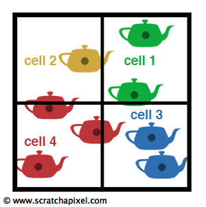
Figure 4: an octree in two dimensions is a quadtree. The node is divided into four cells, and objects are inserted in the cell they overlap. The process of subdividing the cells can be repeated as many times as we want. For example until there is one object per cell or when we have reached a maximum user-defined depth.