基于神经网络（多层感知机）识别手写数字

数据集是经典的MNIST,来自美国国家标准与技术研究所，是人工书写的0~9数字图片，图片的像素为28*28，图片为灰度图。MNIST分别为训练集和测试集，训练数据包含6万个样本，测试数据集包含1万个样本。使用Tensorflow框架加载数据集。

加载数据集的代码如下：

import tensorflow as tf
import  ssl
ssl._create_default_https_context=ssl._create_unverified_context
from tensorflow.examples.tutorials.mnist import  input_data
mnist=input_data.read_data_sets("./mnist_data",one_hot=True)

定义学习率、迭代次数、批大小、批数量（总样本数处以批大小）等参数，设置输入层大小为784，即将28*28的像素展开为一维行向量（一个输入图片784个值）。第一层和第二层隐层神经元数量均为256，输出层的分类类别为0~9的数字，即10个类别。

learning_rate=0.005 #学习率
training_epochs=20 #迭代次数
batch_size=100  #批大小
batch_count=int(mnist.train.num_examples/batch_size) #批数量
n_hidden_1=256 #第一层和第二层隐层神经元数量均为256
n_hidden_2=256
n_input=784#设置输入层的大小为784
n_classes=10 #(0-9数字)
X=tf.placeholder("float",[None,n_input])
Y=tf.placeholder("float",[None,n_classes])

使用tf.random_normal()生成模型权重值参数矩阵和偏置值参数,并将其分别存储于weights和biases变量中，并定义多层感知机的神经网络模型。

weights={
    'weight1':tf.Variable(tf.random_normal([n_input,n_hidden_1])),
    'weight2':tf.Variable(tf.random_normal([n_hidden_1,n_hidden_2])),
    'out':tf.Variable(tf.random_normal([n_hidden_2,n_classes]))
}
biases={
    'bias1':tf.Variable(tf.random_normal([n_hidden_1])),
    'bias2':tf.Variable(tf.random_normal([n_hidden_2])),
    'out':tf.Variable(tf.random_normal([n_classes]))
}
def multilayer_perceptron_model(x):
    layer_1=tf.add(tf.matmul(x,weights['weight1']),biases['bias1'])
    layer_2=tf.add(tf.matmul(layer_1,weights['weight2']),biases['bias2'])
    out_layer=tf.matmul(layer_2,weights['out'])+biases['out']
    return out_layer

使用输入变量X初始化模型，定义损失函数为交叉熵，采用梯度下降法作为优化器，并对模型中tf.placeholder定义的各参数初始化，代码如下:

logits=multilayer_perceptron_model(X) #多层感知机
loss_op=tf.reduce_mean(tf.nn.softmax_cross_entropy_with_logits(logits=logits,labels=Y)) #定义损失函数为交叉熵
optimizer=tf.train.GradientDescentOptimizer(learning_rate)
train_op=optimizer.minimize(loss_op)
init=tf.global_variables_initializer()#参数初始化

将训练集输入模型进行训练，并计算每个批次的平均损失，在每次迭代时输出模型的平均损失，代码如下:

with tf.Session() as sess:
    sess.run(init)
    for epochs in range(training_epochs):
        avg_cost=0
        for i in range(batch_count):
          train_x,train_y=mnist.train.next_batch(batch_size)
          _,c=sess.run([train_op,loss_op],feed_dict={X:train_x,Y:train_y})
          avg_cost+=c/batch_count #计算每个批次的平均损失
        print("Epoch:",'%02d' % (epochs+1),"avg cost={:.6f}".format(avg_cost))

模型训练完成，使用测试集样本对其评估，并计算其正确率，代码如下：

 pred=tf.nn.softmax(logits)  #Apply softmax to logits
    correct_pediction=tf.equal(tf.argmax(pred,1),tf.argmax(Y,1))
    accuracy=tf.reduce_mean(tf.cast(correct_pediction,"float"))
    print("Accuracy:",accuracy.eval({X:mnist.test.images,Y:mnist.test.labels}))

完整代码如下所示:

import tensorflow as tf
import  ssl
ssl._create_default_https_context=ssl._create_unverified_context
from tensorflow.examples.tutorials.mnist import  input_data
mnist=input_data.read_data_sets("./mnist_data",one_hot=True)
#定义学习率、迭代次数、批大小、批数量(总样本数除以批大小)等参数，设置输入层大小为784，即将28*28的像素展开为一维行向量(一个输入图片784个值)。第一层和第二层隐层神经元数量均为256输出层的分类类别为0~9的数字，即10个类别
learning_rate=0.005 #学习率
training_epochs=20 #迭代次数
batch_size=100  #批大小
batch_count=int(mnist.train.num_examples/batch_size) #批数量
n_hidden_1=256 #第一层和第二层隐层神经元数量均为256
n_hidden_2=256
n_input=784#设置输入层的大小为784
n_classes=10 #(0-9数字)
X=tf.placeholder("float",[None,n_input])
Y=tf.placeholder("float",[None,n_classes])
#使用tf.random_normal()生成模型权重值参数矩阵和偏置参数，并将其分别存储于weights和biases变量中，并定义多层感知机的神经网络模型
weights={
    'weight1':tf.Variable(tf.random_normal([n_input,n_hidden_1])),
    'weight2':tf.Variable(tf.random_normal([n_hidden_1,n_hidden_2])),
    'out':tf.Variable(tf.random_normal([n_hidden_2,n_classes]))
}
biases={
    'bias1':tf.Variable(tf.random_normal([n_hidden_1])),
    'bias2':tf.Variable(tf.random_normal([n_hidden_2])),
    'out':tf.Variable(tf.random_normal([n_classes]))
}
def multilayer_perceptron_model(x):
    layer_1=tf.add(tf.matmul(x,weights['weight1']),biases['bias1'])
    layer_2=tf.add(tf.matmul(layer_1,weights['weight2']),biases['bias2'])
    out_layer=tf.matmul(layer_2,weights['out'])+biases['out']
    return out_layer
#使用输入变量X初始化模型，定义损失函数为交叉熵，采用梯度下降法作为优化器(除此之外  还可选MomentumOptimizer、AdagradOptimizer、AdamOptimizer等，见注释部分
#并对模型中tf.placeholder定义的各参数初始化
logits=multilayer_perceptron_model(X) #多层感知机
loss_op=tf.reduce_mean(tf.nn.softmax_cross_entropy_with_logits(logits=logits,labels=Y)) #定义损失函数为交叉熵
optimizer=tf.train.GradientDescentOptimizer(learning_rate)
train_op=optimizer.minimize(loss_op)
init=tf.global_variables_initializer()#参数初始化
#将训练集样本输入模型进行训练，并计算每个批次的平均损失，在每次迭代时输出模型的平均损失
with tf.Session() as sess:
    sess.run(init)
    for epochs in range(training_epochs):
        avg_cost=0
        for i in range(batch_count):
          train_x,train_y=mnist.train.next_batch(batch_size)
          _,c=sess.run([train_op,loss_op],feed_dict={X:train_x,Y:train_y})
          avg_cost+=c/batch_count #计算每个批次的平均损失
        print("Epoch:",'%02d' % (epochs+1),"avg cost={:.6f}".format(avg_cost))
#模型训练完成，使用测试集样本对其评估，并计算其正确率
    pred=tf.nn.softmax(logits)  #Apply softmax to logits
    correct_pediction=tf.equal(tf.argmax(pred,1),tf.argmax(Y,1))
    accuracy=tf.reduce_mean(tf.cast(correct_pediction,"float"))
    print("Accuracy:",accuracy.eval({X:mnist.test.images,Y:mnist.test.labels}))

运行结果如下所示:

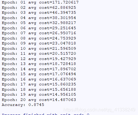
模型的精确率为87%

基于神经网络（多层感知机）识别手写数字

猜你喜欢