numpy与pytorch实现回归

本文通过实现简单的回归来入门下numpy与pytorch
dataSet文末给出

线性回归

线性回归是个古老的问题了，对于线性回归，就是简单找到一组w使得目标函数能最好的拟合数据集X，这个好定义为总均方误差最小。线性回归的解析解数学课本已经给出，证明也不困难，简单的解一个矩阵方程即可。具体可见https://blog.csdn.net/Fleurdalis/article/details/54931721，
一个关键点是矩阵求导法则，除此之外就仅为一个简单的求最值问题

numpy版本

这里用纯numpy以梯度下降求一下

#! python3
# -*- coding:utf-8 -*-
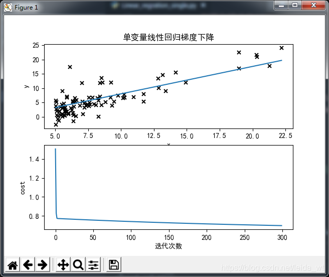
# 单变量线性回归 梯度下降法
import numpy as np
import pandas as pd
import matplotlib.pyplot as plt

plt.rcParams['font.sans-serif'] = ['SimHei']  # 用来正常显示中文标签
plt.rcParams['axes.unicode_minus'] = False  # 用来正常显示负号


class Linear_regration_single:
    def __init__(self, data, alpha=0.01, theta=None, step=1500):
        """初始化线性回归类

        Arguments:
            data {str} -- 数据集地址

        Keyword Arguments:
            alpha {float} -- 学习步长 (default: {None})
            theta {float} -- 起始theta[t0,t1] (default: {None})
            step {int} -- 迭代步数 (default: {None})
        """

        self.cost_history = []
        self.df = pd.read_csv(data)
        self.m = len(self.df)  # 数据总数
        # 学习率
        self.alpha = alpha
        # thetas
        if theta is None:
            self.theta = np.array([0, 0]).reshape(2, 1)
        else:
            self.theta = np.array(theta).reshape(2, 1)
        # 迭代数量
        self.steps = step

        self.x = np.array(self.df['x']).reshape(self.m, 1)
        self.y = np.array(self.df['y']).reshape(self.m, 1)
        self.X = np.hstack((np.ones((self.m, 1)), self.x))  # 补充为其次形式

    def h(self):
        """预测函数

        Returns:
            np.array -- θ0+θ1*x向量
        """

        return np.dot(self.X, self.theta)

    def predict(self, x):
        """预测函数对外接口

        Arguments:
            x {float} -- x值

        Returns:
            y -- 预测
        """

        return self.theta[0, 0]+self.theta[1, 0]*x

    def J(self, theta=None):
        """cost function

        Returns:
            float -- cost
        """
        if theta is None:
            # 默认内部theta
            return np.sum((self.h()-self.y)**2)/(2*self.m)
        else:
            # 计算给定的theta cost
            return np.sum((np.dot(self.X, theta)-self.y)**2)/(2*self.m)

    def descend_gradient(self):
        """以梯度下降更新theta
        """
        for i in range(self.steps):
            #print(self.theta, self.J())
            self.cost_history.append(self.J())  # 记录cost
            # 更新theta
            derta = np.dot(self.X.T, (self.h()-self.y))*self.alpha/self.m
            self.theta = self.theta-derta

    def closed_solution(self):
        """封闭解

        Returns:
            np.array -- theta封闭解
        """

        from numpy.linalg import inv
        return np.dot(np.dot(inv(np.dot(self.X.T, self.X)), self.X.T), self.y)

    def plot(self):
        """绘制结果
        """

        fig = plt.figure()
        ax1 = fig.add_subplot(211)  # 高1 宽2 图号1
        ax2 = fig.add_subplot(212)  # 高1 宽2 图号2
        ax1.scatter(self.x, self.y, label='skitscat',
                    color='k', s=25, marker="x")
        line_x = [min(self.x), max(self.x)]
        line_y = [self.predict(x) for x in line_x]
        ax1.plot(line_x, line_y)
        ax1.set_xlabel('x')
        ax1.set_ylabel('y')
        ax2.plot(self.cost_history)
        ax2.set_xlabel('迭代次数')
        ax2.set_ylabel('cost')
        ax1.set_title('单变量线性回归梯度下降')
        plt.show()

    def info(self):
        print('decent method solution:')
        print('final cost: '+str(self.J()))
        print('theat: '+str(self.theta))
        print('closed solution:')
        print('final cost: '+str(self.J(self.closed_solution())))
        print('theat: '+str(self.closed_solution()))


if __name__ == "__main__":
    data_dir = './ex1data1.txt'
    t = Linear_regration_single(data_dir)
    t.descend_gradient()
    t.info()
    t.plot()

可观测到与封闭解的结果还是很接近的
decent method solution:
final cost: 4.964362046184745
theat: [[-1.58199122]
[ 0.96058838]]
closed solution:
final cost: 4.476971375975179
theat: [[-3.89578088]
[ 1.19303364]]
在这里插入图片描述

pytorch版本

pytorch version=0.4.1
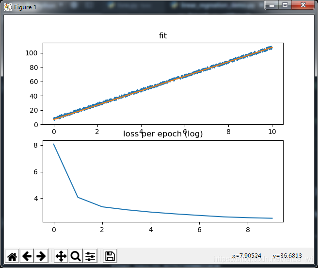
下面的版本是以pytorch实现的，借助自动求导，只要定义好前向计算方法和loss即可。

import numpy as np
import torch.utils.data
import torch as t
import matplotlib.pyplot as plt
t.manual_seed(1)    # reproducible
fig = plt.figure()
# 首先造出来一些带噪声的数据
N = 1100
x = t.linspace(0, 10, N)
y = 10*x+5+t.rand(N)*5
ax1 = fig.add_subplot(211)  # 高2 宽2 图号1
ax1.plot(x.numpy(), y.numpy())
# 从Tensor构建DataSet对象
data = t.utils.data.TensorDataset(x, y)
# 随机分割数据集，测试集
train, test = t.utils.data.random_split(data, [1000, 100])
# 建立dataloader shuffle来使得每个epoch前打乱数据
trainloader = t.utils.data.DataLoader(train, batch_size=100, shuffle=True)
testloader = t.utils.data.DataLoader(test, batch_size=100, shuffle=True)

# 定义模型参数 for y_head=w@x+b
w = t.rand(1, 1, requires_grad=True)
b = t.zeros(1, 1, requires_grad=True)

optimizer = t.optim.SGD([w, b], lr=0.03, momentum=0.6)
#optimizer = t.optim.Adam([w,b],lr=10)
loss_his = []
batch_loss = 0
for epoch in range(10):
    for i, (bx, by) in enumerate(trainloader):
        bx = bx.view(1, -1)  # torch.Size([100])->torch.Size([1,100])
        y_head = w@bx+b

        loss = 0.5*(y_head-by)**2
        loss = loss.mean()
        batch_loss += loss.item()

        optimizer.zero_grad()  # 先清除梯度
        loss.backward()
        optimizer.step()
        #print('training:epoch {} batch {}'.format(epoch,i))
    loss_his.append(batch_loss)
    batch_loss = 0


def main():
    print('w={},b={}'.format(w.item(), b.item()))
    y_head = w*x+b
    ax1.plot(x.numpy(), y_head.detach().numpy().flatten())
    ax1.set_title('fit')
    print('final_loss={}'.format(loss_his[-1]))
    ax2 = fig.add_subplot(212)  # 高2 宽2 图号2
    ax2.set_title('loss per epoch (log)')
    ax2.plot(np.log(loss_his))
    plt.show()


if __name__ == '__main__':
    main()

在这里插入图片描述

pytorch神经网络回归

借助神经网络的强大非线性能力，可以对任意曲线拟合，下面以拟合sin函数为例，定义了简单的全连接神经网络解决问题。
这里训练采用全局训练，未取batch
此外观察到采用BatchNorm之后训练稳定性明显提高，收敛略有提速

import numpy as np
import math
import matplotlib.pyplot as plt
import torch as t
from torch import nn, optim
import torch.utils.data
import torch.nn.functional as F

N = 1000
x = t.linspace(0, 2*np.pi, N)
y = t.sin(x)
#y = t.sin(x)+t.randn(len(x))/30
print('x.shape, y.shape:', x.shape, y.shape)

t.manual_seed(1)


class Dense(nn.Module):
    # 自定义全连接层
    def __init__(self, inshape, outshape):
        super(Dense, self).__init__()
        # 这里对w采用Xavier初始化（实为变种，仅考虑输入尺寸，这为普遍做法）
        alpha = 1./math.sqrt(inshape)
        self.w = nn.Parameter(t.randn(inshape, outshape)*alpha)
        # 偏置的初始化0即可
        self.b = nn.Parameter(t.zeros(outshape))

    def forward(self, x):
        return x@self.w+self.b


class NN(nn.Module):
    def __init__(self, useDense=True):
        super(NN, self).__init__()
        if useDense:
            # 使用自定义的全连接层
            self.l1 = Dense(1, 20)
            self.l2 = Dense(20, 40)
            self.l3 = Dense(40, 1)
        else:
            self.l1 = nn.Linear(1, 20)
            self.l2 = nn.Linear(20, 40)
            self.l3 = nn.Linear(40, 1)
        self.BN1 = nn.BatchNorm1d(20)
        self.BN2 = nn.BatchNorm1d(40)

    def forward(self, x):
        out = self.l1(x.view(-1, 1))
        out = self.BN1(out)
        out = F.relu(out)
        out = self.l2(out)
        out = self.BN2(out)
        out = F.relu(out)
        out = self.l3(out)
        return out

    def predict(self, x):
        with t.no_grad():
            return self.forward(x)


net = NN()
iter_num = 500
criterion = nn.MSELoss()
#optimizer = optim.SGD(net.parameters(), lr=0.0005, momentum=0.9)
optimizer = optim.Adam(net.parameters(), lr=0.07)
loss_his = []
net.train()
for epoch in range(iter_num):
    y_head = net.forward(x)
    loss = criterion(y_head.view(-1), y)
    loss_his.append(loss.item())
    if loss.item() < 1e-5:
        print('epoch=', epoch)
        break
    net.zero_grad()
    loss.backward()
    optimizer.step()
net.eval()
print('final loss:{}'.format(loss_his[-1]))
fig = plt.figure()
f1 = fig.add_subplot(211)
f2 = fig.add_subplot(212)
f1.plot(np.log10(np.array(loss_his)))

y_head = net.predict(x)
f2.plot(y.numpy())
f2.plot(y_head.numpy())
plt.show()

在这里插入图片描述
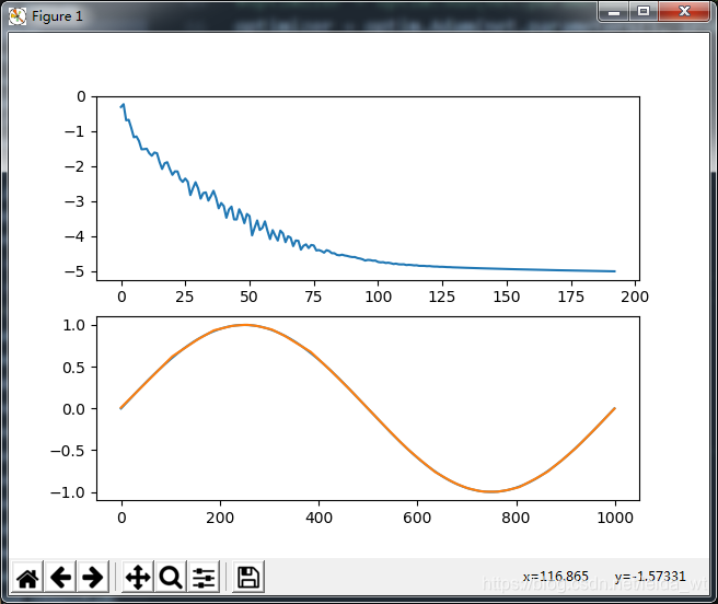
epoch= 192
final loss:9.999754183809273e-06

总结

numpy的shape=(3,)与shape=(3,1)的数据是不同的，这在numpy中常会错，可考虑assert或注意归并操作的keepdim。
numpy的sum等归并操作默认丢弃维数为1的维度，可指定keepdim=True或使用reshape方法。reshape不移动数据而是生成新的观察数据的方式，开销很小。
plt.rcParams[‘font.sans-serif’] = [‘SimHei’] # 用来正常显示中文标签
plt.rcParams[‘axes.unicode_minus’] = False # 用来正常显示符号
对cost曲线取对数可看的更清楚些
pytorch view 与 numpy的reshape等价，不会幅复制数据
pytorch取计算图的Tensor并转numpy要注意先从计算图上取下，即调用detach方法
数据的归一化效果显著
对于pytorch里不需要记录梯度的计算，采用no_grad

def predict(self, x):
        with t.no_grad():
            return self.forward(x)

numpy的计算值可用到单一cpu核，pytorch的blas后端已经做好了并行，通常可满载
data来自cs229的coursera板
链接: https://pan.baidu.com/s/1ibqIBTB7qTcq69EQ4qWcSw 提取码: 4jem