pytorch 实现线性回归

实现线性回归

线性回归是机器学习入门知识，应用十分广泛。线性回归利用数理统计中回归分析，来确定两种或两种以上变量间相互依赖的定量关系的，其表达形式为 $y = wx+b+e$， $e$为误差服从均值为0的正态分布。首先让我们来确认线性回归的损失函数：
$loss = \sum_i^N \frac 1 2 ({y_i-(wx_i+b)})^2$
然后利用随机梯度下降法更新参数 $\textbf{w}$和 $\textbf{b}$来最小化损失函数，最终学得 $\textbf{w}$和 $\textbf{b}$的数值。

import torch as t
%matplotlib inline
from matplotlib import pyplot as plt
from IPython import display

device = t.device('cpu') #如果你想用gpu，改成t.device('cuda:0')

# 设置随机数种子，保证在不同电脑上运行时下面的输出一致
t.manual_seed(1000) 

def get_fake_data(batch_size=8):
    ''' 产生随机数据：y=x*2+3，加上了一些噪声'''
    x = t.rand(batch_size, 1, device=device) * 5
    y = x * 2 + 3 +  t.randn(batch_size, 1, device=device)
    return x, y

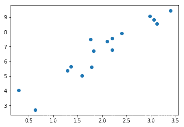
# 来看看产生的x-y分布
x, y = get_fake_data(batch_size=16)
plt.scatter(x.squeeze().cpu().numpy(), y.squeeze().cpu().numpy())

<matplotlib.collections.PathCollection at 0x7fb5f2e5f780>

# 随机初始化参数
w = t.rand(1, 1).to(device)
b = t.zeros(1, 1).to(device)
lr =0.02 # 学习率
for ii in range(500):
    x, y = get_fake_data(batch_size=4)
    # forward：计算loss
    y_pred = x.mm(w) + b.expand_as(y) # x@W等价于x.mm(w);for python3 only
    loss = 0.5 * (y_pred - y) ** 2 # 均方误差
    loss = loss.mean() 
    # backward：手动计算梯度
    dloss = 1
    dy_pred = dloss * (y_pred - y)
    dw = x.t().mm(dy_pred)
    db = dy_pred.sum()
    # 更新参数
    w.sub_(lr * dw)
    b.sub_(lr * db)
    if ii%50 ==0:
        # 画图
        display.clear_output(wait=True)
        x = t.arange(0, 6).view(-1, 1)
        y = x.mm(w) + b.expand_as(x)
        plt.plot(x.cpu().numpy(), y.cpu().numpy()) # predicted
        x2, y2 = get_fake_data(batch_size=32) 
        plt.scatter(x2.numpy(), y2.numpy()) # true data  
        plt.xlim(0, 5)
        plt.ylim(0, 13)
        plt.show()
        plt.pause(0.5)    
print('w: ', w.item(), 'b: ', b.item())

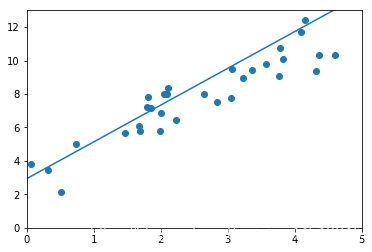
w:  1.9115010499954224 b:  3.044184446334839

w=2、b=3，图中直线和数据已经实现较好的拟合。