import numpy as np # 快速操作结构数组的工具
import matplotlib.pyplot as plt  # 可视化绘制
from sklearn.linear_model import RidgeCV  # Ridge岭回归,RidgeCV带有广义交叉验证的岭回归
from sklearn.preprocessing import PolynomialFeatures  # 使数据具有多项式特征


# 生成数据
x = np.arange(-2, 2, 0.1)
y = -x**3 + 2*x**2 - 3*x + 1 + np.random.rand()*2

x = x.reshape((40, 1))

# 加入多项式特征,否则默认为一次
poly_reg = PolynomialFeatures(4)  # 最高为4次
x_train = poly_reg.fit_transform(x)

# 声明模型 训练模型
Rid_model = RidgeCV(alphas=[0.1, 0.5, 1, 10])
Rid_model.fit(x_train, y)

# 形成新数据
x_2 = np.arange(-5, 5, 0.1)
y_result = -x_2**3 + 2*x_2**2 - 3*x_2 + 1  # 希望得到的预期结果

# 使用模型预测
x_2 = x_2.reshape((100, 1))
x_pre = poly_reg.fit_transform(x_2)
y_predict = Rid_model.predict(x_pre)  # 预测结果

# 绘制散点图
plt.scatter(x_2, y_result, marker='x', color='blue')
plt.scatter(x, y, marker='x', color='green')
plt.plot(x_2, y_predict, c='r')

# 绘制x轴和y轴坐标
plt.xlabel("x")
plt.ylabel("y")

# 显示图形
plt.show()
运行结果如下:
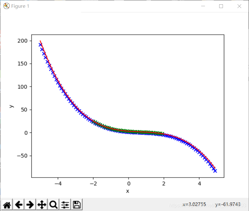
可以看到,拟合曲线(红色)和期望图像(蓝色的点)大致相同。