Python Sklearn库常用操作

  Python sklearn库是一个丰富的机器学习库，里面包含内容太多，这里对一些工程里常用的操作做个简要的概述，以后还会根据自己用的进行更新。

---

1、LabelEncoder

简单来说 LabelEncoder 是对不连续的数字或者文本进行按序编号，可以用来生成属性/标签

from sklearn.preprocessing import LabelEncoder
encoder=LabelEncoder()
encoder.fit([1,3,2,6])
t=encoder.transform([1,6,6,2])
print(t)

输出： [0 3 3 1]

---

2、OneHotEncoder

OneHotEncoder 用于将表示分类的数据扩维，将[[1]，[2]，[3]，[4]]映射为 0,1,2,3的位置为1（高维的数据自己可以测试）：

from sklearn.preprocessing import OneHotEncoder
oneHot=OneHotEncoder()#声明一个编码器
oneHot.fit([[1],[2],[3],[4]])
print(oneHot.transform([[2],[3],[1],[4]]).toarray())

输出：[[0. 1. 0. 0.]
 [0. 0. 1. 0.]
 [1. 0. 0. 0.]
 [0. 0. 0. 1.]]
正如keras中的keras.utils.to_categorical(y_train, num_classes)

---

.

3、sklearn.model_selection.train_test_split随机划分训练集和测试集

一般形式： 
train_test_split是交叉验证中常用的函数，功能是从样本中随机的按比例选取train data和testdata，形式为：

X_train,X_test, y_train, y_test =train_test_split(train_data,train_target,test_size=0.2, train_size=0.8,random_state=0)

参数解释： 
- train_data：所要划分的样本特征集 
- train_target：所要划分的样本结果 
- test_size：测试样本占比，如果是整数的话就是样本的数量 

-train_size：训练样本的占比，（注：测试占比和训练占比任写一个就行）
- random_state：是随机数的种子。 
- 随机数种子：其实就是该组随机数的编号，在需要重复试验的时候，保证得到一组一样的随机数。比如你每次都填1，其他参数一样的情况下你得到的随机数组是一样的。但填0或不填，每次都会不一样。 
随机数的产生取决于种子，随机数和种子之间的关系遵从以下两个规则： 
- 种子不同，产生不同的随机数；种子相同，即使实例不同也产生相同的随机数。

from sklearn.model_selection import train_test_split
from sklearn.datasets import load_iris
iris=load_iris()
train=iris.data
target=iris.target
# 避免过拟合，采用交叉验证，验证集占训练集20%，固定随机种子（random_state)
train_X,test_X, train_y, test_y = train_test_split(train,
                                                   target,
                                                   test_size = 0.2,
                                                   random_state = 0)
print(train_y.shape)

得到的结果数据：train_X : 训练集的数据,train_Y：训练集的标签，对应test 为测试集的数据和标签

---

4、pipeline

本节参考与文章：用 Pipeline 将训练集参数重复应用到测试集 
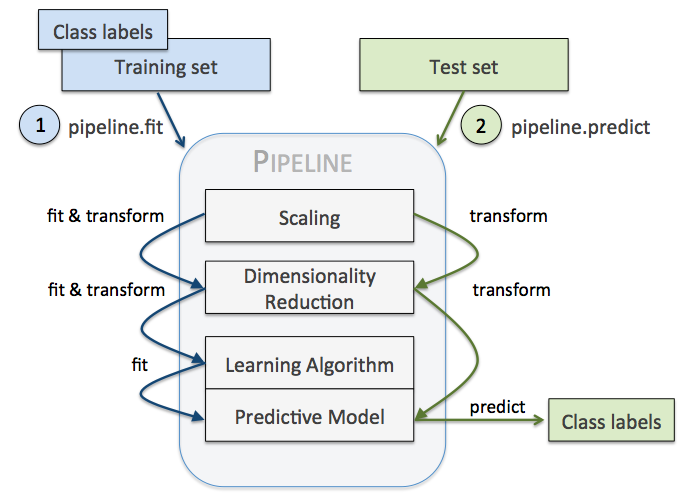
pipeline 实现了对全部步骤的流式化封装和管理，可以很方便地使参数集在新数据集上被重复使用。

pipeline 可以用于下面几处：

• 模块化 Feature Transform，只需写很少的代码就能将新的 Feature 更新到训练集中。
• 自动化 Grid Search，只要预先设定好使用的 Model 和参数的候选，就能自动搜索并记录最佳的 Model。
• 自动化 Ensemble Generation，每隔一段时间将现有最好的 K 个 Model 拿来做 Ensemble。

问题是要对数据集 Breast Cancer Wisconsin 进行分类， 
该数据集包含 569 个样本，第一列 ID，第二列类别(M=恶性肿瘤，B=良性肿瘤)， 
第 3-32 列是实数值的特征。

我们要用 Pipeline 对训练集和测试集进行如下操作：

• 先用 StandardScaler 对数据集每一列做标准化处理，（是 transformer）
• 再用 PCA 将原始的 30 维度特征压缩的 2 维度，（是 transformer）
• 最后再用模型 LogisticRegression。（是 Estimator）
• 调用 Pipeline 时，输入由元组构成的列表，每个元组第一个值为变量名，元组第二个元素是 sklearn 中的 transformer 
  或 Estimator。

注意中间每一步是 transformer，即它们必须包含 fit 和 transform 方法，或者 fit_transform。 
最后一步是一个 Estimator，即最后一步模型要有 fit 方法，可以没有 transform 方法。

然后用 Pipeline.fit对训练集进行训练，pipe_lr.fit(X_train, y_train) 
再直接用 Pipeline.score 对测试集进行预测并评分 pipe_lr.score(X_test, y_test)

import pandas as pd
from sklearn.model_selection import train_test_split
from sklearn.preprocessing import LabelEncoder
from sklearn.preprocessing import StandardScaler
from sklearn.decomposition import PCA
from sklearn.linear_model import LogisticRegression

from sklearn.pipeline import Pipeline
#需要联网
df = pd.read_csv('http://archive.ics.uci.edu/ml/machine-learning-databases/breast-cancer-wisconsin/wdbc.data',
                 header=None)
                                 # Breast Cancer Wisconsin dataset
X, y = df.values[:, 2:], df.values[:, 1]
encoder = LabelEncoder()
y = encoder.fit_transform(y)
X_train, X_test, y_train, y_test = train_test_split(X, y, test_size=.2, random_state=0)
pipe_lr = Pipeline([('sc', StandardScaler()),
                    ('pca', PCA(n_components=2)),
                    ('clf', LogisticRegression(random_state=1))
                    ])
pipe_lr.fit(X_train, y_train)
print('Test accuracy: %.3f' % pipe_lr.score(X_test, y_test))

还可以用来选择特征：

例如用 SelectKBest 选择特征， 
分类器为 SVM，

anova_filter = SelectKBest(f_regression, k=5)
clf = svm.SVC(kernel='linear')
anova_svm = Pipeline([('anova', anova_filter), ('svc', clf)])

当然也可以应用 K-fold cross validation：

Pipeline 的工作方式：

当管道 Pipeline 执行 fit 方法时， 
首先 StandardScaler 执行 fit 和 transform 方法， 
然后将转换后的数据输入给 PCA， 
PCA 同样执行 fit 和 transform 方法， 
再将数据输入给 LogisticRegression，进行训练。 

5 perdict 直接返回预测值，predict_proba返回每组数据预测值的概率，每行的概率和为1，如训练集/测试集有 下例中的两个类别，测试集有三个，则 predict返回的是一个 3*1的向量，而 predict_proba 返回的是 3*2维的向量，如下结果所示。

# conding :utf-8
from sklearn.linear_model import LogisticRegression
import numpy as np

x_train = np.array([[1, 2, 3],
                    [1, 3, 4],
                    [2, 1, 2],
                    [4, 5, 6],
                    [3, 5, 3],
                    [1, 7, 2]])

y_train = np.array([3, 3, 3, 2, 2, 2])

x_test = np.array([[2, 2, 2],
                   [3, 2, 6],
                   [1, 7, 4]])

clf = LogisticRegression()
clf.fit(x_train, y_train)

# 返回预测标签
print(clf.predict(x_test))

# 返回预测属于某标签的概率
print(clf.predict_proba(x_test))

---

4、10+款机器学习算法对比

Sklearn API：http://scikit-learn.org/stable/modules/classes.html#module-sklearn.ensemble

4.1 生成数据

import numpy as np
np.random.seed(10)
%matplotlib inline 
import matplotlib.pyplot as plt
import pandas as pd
from sklearn.datasets import make_classification
from sklearn.linear_model import LogisticRegression
from sklearn.ensemble import (RandomTreesEmbedding, RandomForestClassifier,
                              GradientBoostingClassifier)
from sklearn.preprocessing import OneHotEncoder
from sklearn.model_selection import train_test_split
from sklearn.metrics import roc_curve,accuracy_score,recall_score
from sklearn.pipeline import make_pipeline
from sklearn.calibration import calibration_curve
import copy
print(__doc__)
from matplotlib.colors import ListedColormap
from sklearn.model_selection import train_test_split
from sklearn.preprocessing import StandardScaler
from sklearn.datasets import make_moons, make_circles, make_classification
from sklearn.neural_network import MLPClassifier
from sklearn.neighbors import KNeighborsClassifier
from sklearn.svm import SVC
from sklearn.gaussian_process import GaussianProcessClassifier
from sklearn.gaussian_process.kernels import RBF
from sklearn.tree import DecisionTreeClassifier
from sklearn.ensemble import RandomForestClassifier, AdaBoostClassifier
from sklearn.naive_bayes import GaussianNB
from sklearn.discriminant_analysis import QuadraticDiscriminantAnalysis

# 数据
X, y = make_classification(n_samples=100000)
X_train, X_test, y_train, y_test = train_test_split(X, y, test_size=0.2,random_state = 4000)  # 对半分
X_train, X_train_lr, y_train, y_train_lr = train_test_split(X_train,
                                                            y_train,
                                                            test_size=0.2,random_state = 4000)
print(X_train.shape, X_test.shape, y_train.shape, y_test.shape)

def yLabel(y_pred):
    y_pred_f = copy.copy(y_pred)
    y_pred_f[y_pred_f>=0.5] = 1
    y_pred_f[y_pred_f<0.5] = 0
    return y_pred_f

def acc_recall(y_test, y_pred_rf):
    return {'accuracy': accuracy_score(y_test, yLabel(y_pred_rf)), \
            'recall': recall_score(y_test, yLabel(y_pred_rf))}

4.2 八款主流机器学习模型

h = .02  # step size in the mesh
names = ["Nearest Neighbors", "Linear SVM", "RBF SVM",
         "Decision Tree", "Neural Net", "AdaBoost",
         "Naive Bayes", "QDA"]
# 去掉"Gaussian Process"，太耗时，是其他的300倍以上

classifiers = [
    KNeighborsClassifier(3),
    SVC(kernel="linear", C=0.025),
    SVC(gamma=2, C=1),
    #GaussianProcessClassifier(1.0 * RBF(1.0)),
    DecisionTreeClassifier(max_depth=5),
    #RandomForestClassifier(max_depth=5, n_estimators=10, max_features=1),
    MLPClassifier(alpha=1),
    AdaBoostClassifier(),
    GaussianNB(),
    QuadraticDiscriminantAnalysis()]

predictEight = {}
for name, clf in zip(names, classifiers):
    predictEight[name] = {}
    predictEight[name]['prob_pos'],predictEight[name]['fpr_tpr'],predictEight[name]['acc_recall'] = [],[],[]
    predictEight[name]['importance'] = []
    print('\n --- Start Model : %s ----\n'%name)
    %time clf.fit(X_train, y_train)
    # 一些计算决策边界的模型 计算decision_function
    if hasattr(clf, "decision_function"):
        %time prob_pos = clf.decision_function(X_test)
        # # The confidence score for a sample is the signed distance of that sample to the hyperplane.
    else:
        %time prob_pos= clf.predict_proba(X_test)[:, 1]
        prob_pos = (prob_pos - prob_pos.min()) / (prob_pos.max() - prob_pos.min())
        # 需要归一化
    predictEight[name]['prob_pos'] = prob_pos

    # 计算ROC、acc、recall
    predictEight[name]['fpr_tpr'] = roc_curve(y_test, prob_pos)[:2]
    predictEight[name]['acc_recall'] = acc_recall(y_test, prob_pos)  # 计算准确率与召回

    # 提取信息
    if hasattr(clf, "coef_"):
        predictEight[name]['importance'] = clf.coef_
    elif hasattr(clf, "feature_importances_"):
        predictEight[name]['importance'] = clf.feature_importances_
    elif hasattr(clf, "sigma_"):
        predictEight[name]['importance'] = clf.sigma_
        # variance of each feature per class 在朴素贝叶斯之中体现

结果输出类似：

Automatically created module for IPython interactive environment

 --- Start Model : Nearest Neighbors ----

CPU times: user 103 ms, sys: 0 ns, total: 103 ms
Wall time: 103 ms
CPU times: user 2min 8s, sys: 3.43 ms, total: 2min 8s
Wall time: 2min 9s

 --- Start Model : Linear SVM ----

CPU times: user 25.4 s, sys: 149 ms, total: 25.6 s
Wall time: 25.6 s
CPU times: user 3.47 s, sys: 1.23 ms, total: 3.47 s
Wall time: 3.47 s

4.3 树模型 - 随机森林

案例地址：http://scikit-learn.org/stable/auto_examples/ensemble/plot_feature_transformation.html#sphx-glr-auto-examples-ensemble-plot-feature-transformation-py

'''
model 0 : lm
logistic
'''
print('LM 开始计算...')
lm = LogisticRegression()
%time lm.fit(X_train, y_train)
y_pred_lm = lm.predict_proba(X_test)[:, 1]
fpr_lm, tpr_lm, _ = roc_curve(y_test, y_pred_lm)
lm_ar = acc_recall(y_test, y_pred_lm)  # 计算准确率与召回

'''
model 1 : rt + lm
无监督变换 + lg
'''
# Unsupervised transformation based on totally random trees
print('随机森林编码+LM 开始计算...')


rt = RandomTreesEmbedding(max_depth=3, n_estimators=n_estimator,
    random_state=0)
# 数据集的无监督变换到高维稀疏表示。

rt_lm = LogisticRegression()
pipeline = make_pipeline(rt, rt_lm)
%time pipeline.fit(X_train, y_train)
y_pred_rt = pipeline.predict_proba(X_test)[:, 1]
fpr_rt_lm, tpr_rt_lm, _ = roc_curve(y_test, y_pred_rt)
rt_lm_ar = acc_recall(y_test, y_pred_rt)  # 计算准确率与召回

'''
model 2 : RF / RF+LM
'''
print('\n 随机森林系列 开始计算... ')

# Supervised transformation based on random forests
rf = RandomForestClassifier(max_depth=3, n_estimators=n_estimator)
rf_enc = OneHotEncoder()
rf_lm = LogisticRegression()
rf.fit(X_train, y_train)
rf_enc.fit(rf.apply(X_train))  # rf.apply(X_train)-(1310, 100)     X_train-(1310, 20)
# 用100棵树的信息作为X，载入做LM模型
%time rf_lm.fit(rf_enc.transform(rf.apply(X_train_lr)), y_train_lr)

y_pred_rf_lm = rf_lm.predict_proba(rf_enc.transform(rf.apply(X_test)))[:, 1]
fpr_rf_lm, tpr_rf_lm, _ = roc_curve(y_test, y_pred_rf_lm)
rf_lm_ar = acc_recall(y_test, y_pred_rf_lm)  # 计算准确率与召回

'''
model 2 : GRD / GRD + LM
'''
print('\n 梯度提升树系列 开始计算... ')

grd = GradientBoostingClassifier(n_estimators=n_estimator)
grd_enc = OneHotEncoder()
grd_lm = LogisticRegression()
grd.fit(X_train, y_train)
grd_enc.fit(grd.apply(X_train)[:, :, 0])
%time grd_lm.fit(grd_enc.transform(grd.apply(X_train_lr)[:, :, 0]), y_train_lr)

y_pred_grd_lm = grd_lm.predict_proba(
    grd_enc.transform(grd.apply(X_test)[:, :, 0]))[:, 1]
fpr_grd_lm, tpr_grd_lm, _ = roc_curve(y_test, y_pred_grd_lm)
grd_lm_ar = acc_recall(y_test, y_pred_grd_lm)  # 计算准确率与召回

# The gradient boosted model by itself
y_pred_grd = grd.predict_proba(X_test)[:, 1]
fpr_grd, tpr_grd, _ = roc_curve(y_test, y_pred_grd)
grd_ar = acc_recall(y_test, y_pred_grd)  # 计算准确率与召回


# The random forest model by itself
y_pred_rf = rf.predict_proba(X_test)[:, 1]
fpr_rf, tpr_rf, _ = roc_curve(y_test, y_pred_rf)
rf_ar = acc_recall(y_test, y_pred_rf)  # 计算准确率与召回

输出结果为：

LM 开始计算...
随机森林编码+LM 开始计算...
CPU times: user 591 ms, sys: 85.5 ms, total: 677 ms
Wall time: 574 ms

 随机森林系列 开始计算... 
CPU times: user 76 ms, sys: 0 ns, total: 76 ms
Wall time: 76 ms

 梯度提升树系列 开始计算... 
CPU times: user 60.6 ms, sys: 0 ns, total: 60.6 ms
Wall time: 60.6 ms

4.4 一些结果展示：每个模型的准确率与召回率

# 8款常规模型
for x,y in predictEight.items():
    print('\n ----- The Model  : %s , -----\n '%(x)  )
    print(predictEight[x]['acc_recall'])

# 树模型
names = ['LM','LM + RT','LM + RF','GBT + LM','GBT','RF']
ar_list = [lm_ar,rt_lm_ar,rf_lm_ar,grd_lm_ar,grd_ar,rf_ar]
for x,y in zip(names,ar_list):
    print('\n --- %s 准确率与召回为: ---- \n '%x,y)

结果输出：

 ----- The Model  : Linear SVM , -----
{'recall': 0.84561049445005043, 'accuracy': 0.89100000000000001}
 ---- The Model  : Decision Tree , -----
{'recall': 0.90918264379414737, 'accuracy': 0.89949999999999997}
 ----- The Model  : AdaBoost , -----
{'recall': 0.028254288597376387, 'accuracy': 0.51800000000000002}
 ----- The Model  : Neural Net , -----
{'recall': 0.91523713420787078, 'accuracy': 0.90249999999999997}
 ----- The Model  : Naive Bayes , -----
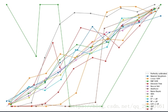
{'recall': 0.91523713420787078, 'accuracy': 0.89300000000000002}

4.5 结果展示：校准曲线

Calibration curves may also be referred to as reliability diagrams. 
可靠性检验的方式。

# #############################################################################
# Plot calibration plots
names = ["Nearest Neighbors", "Linear SVM", "RBF SVM",
         "Decision Tree", "Neural Net", "AdaBoost",
         "Naive Bayes", "QDA"]


plt.figure(figsize=(15, 15))
ax1 = plt.subplot2grid((3, 1), (0, 0), rowspan=2)
ax2 = plt.subplot2grid((3, 1), (2, 0))

ax1.plot([0, 1], [0, 1], "k:", label="Perfectly calibrated")
for prob_pos, name in [[predictEight[n]['prob_pos'],n] for n in names] + [(y_pred_lm,'LM'),
                       (y_pred_rt,'RT + LM'),
                       (y_pred_rf_lm,'RF + LM'),
                       (y_pred_grd_lm,'GBT + LM'),
                       (y_pred_grd,'GBT'),
                       (y_pred_rf,'RF')]:

    prob_pos = (prob_pos - prob_pos.min()) / (prob_pos.max() - prob_pos.min())

    fraction_of_positives, mean_predicted_value = calibration_curve(y_test, prob_pos, n_bins=10)

    ax1.plot(mean_predicted_value, fraction_of_positives, "s-",
             label="%s" % (name, ))

    ax2.hist(prob_pos, range=(0, 1), bins=10, label=name,
             histtype="step", lw=2)

ax1.set_ylabel("Fraction of positives")
ax1.set_ylim([-0.05, 1.05])
ax1.legend(loc="lower right")
ax1.set_title('Calibration plots  (reliability curve)')

ax2.set_xlabel("Mean predicted value")
ax2.set_ylabel("Count")
ax2.legend(loc="upper center", ncol=2)

plt.tight_layout()
plt.show()

第一张图 
fraction_of_positives,每个概率片段,正数的比例= 正数/总数 
Mean predicted value,每个概率片段,正数的平均值 
第二张图 
每个概率分数段的个数

结果展示为： 

4.6 模型的结果展示：重要性输出

大家都知道一些树模型可以输出重要性，回归模型可以输出系数，带有决策平面的（譬如SVM）可以计算点到决策边界的距离。

# 重要性
print('\n -------- RadomFree importances ------------\n')
print(rf.feature_importances_)
print('\n -------- GradientBoosting importances ------------\n')
print(grd.feature_importances_)
print('\n -------- Logistic Coefficient  ------------\n')
lm.coef_ 

# 其他几款模型的特征选择
[[predictEight[n]['importance'],n] for n in names if predictEight[n]['importance'] != [] ]

在本次10+机器学习案例之中，可以看到，可以输出重要性的模型有： 
随机森林rf.feature_importances_ 
GBTgrd.feature_importances_ 
Decision Tree decision.feature_importances_ 
AdaBoost AdaBoost.feature_importances_

可以计算系数的有：线性模型，lm.coef_ 、 SVM svm.coef_

Naive Bayes得到的是：NaiveBayes.sigma_

解释为：variance of each feature per class

4.7 ROC值的计算与plot

plt.figure(1)
plt.plot([0, 1], [0, 1], 'k--')
plt.plot(fpr_lm, tpr_lm, label='LR')
plt.plot(fpr_rt_lm, tpr_rt_lm, label='RT + LR')
plt.plot(fpr_rf, tpr_rf, label='RF')
plt.plot(fpr_rf_lm, tpr_rf_lm, label='RF + LR')
plt.plot(fpr_grd, tpr_grd, label='GBT')
plt.plot(fpr_grd_lm, tpr_grd_lm, label='GBT + LR')
# 8 款模型
for (fpr,tpr),name in [[predictEight[n]['fpr_tpr'],n] for n in names] :
    plt.plot(fpr, tpr, label=name)


plt.xlabel('False positive rate')
plt.ylabel('True positive rate')
plt.title('ROC curve')
plt.legend(loc='best')
plt.show()

plt.figure(2)
plt.xlim(0, 0.2)
plt.ylim(0.4, 1)     # ylim改变     # matt
plt.plot([0, 1], [0, 1], 'k--')
plt.plot(fpr_lm, tpr_lm, label='LR')
plt.plot(fpr_rt_lm, tpr_rt_lm, label='RT + LR')
plt.plot(fpr_rf, tpr_rf, label='RF')
plt.plot(fpr_rf_lm, tpr_rf_lm, label='RF + LR')
plt.plot(fpr_grd, tpr_grd, label='GBT')
plt.plot(fpr_grd_lm, tpr_grd_lm, label='GBT + LR')
for (fpr,tpr),name in [[predictEight[n]['fpr_tpr'],n] for n in names] :
    plt.plot(fpr, tpr, label=name)
plt.xlabel('False positive rate')
plt.ylabel('True positive rate')
plt.title('ROC curve (zoomed in at top left)')
plt.legend(loc='best')
plt.show()