TensorFlow可视化cifar-10卷积后的特征

本文大概步骤：准备数据→搭建网络→训练测试（并添加tensorboard的IMAGES）

目录

准备数据

下载数据集

反序列化数据

调整数据

定义训练、测试的样本和标签

网络搭建及训练测试

网络结构：

输入层：32*32*3 → 32个5*5的三通道卷积核 → 卷积层1:32*32*32 → 3*3步幅为2的池化 → 池化层1:16*16*32 →  64个5*5的64通道卷积核 → 卷积层2:16*16*64 → 3*3步幅为2的池化 → 池化层2:8*8*64 → 全连接层1:384 → 全连接层2:192 → 输出层:10

整体代码

可视化结果

---

准备数据

1. 下载数据集
2. 反序列化数据
3. 调整数据
4. 定义训练、测试的样本和标签

• 下载数据集

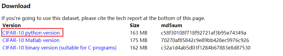
打开官网http://www.cs.toronto.edu/~kriz/cifar.html，找到相应的python版本的数据集进行下载，如下图：（另外也有别的下载方式，import cifar10 cifar10.maybe_download_and_extract()，此处仅做简单介绍，细节请自行百度or谷歌）

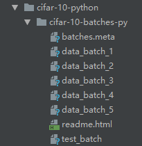
下载好后的数据如下图所示：其中，训练数据为data_batch_1~5，测试数据为test_batch，每个batch为10000幅图像

• 反序列化数据

在官网中给出了相应的反序列化代码：(反序列化后的数据是一个字典，相应的key为：b'filename',b'labels',b'data')

值得一提的是反序列化后的data中的每一个图像为一行数据，共10000行，每行的前1024个值为相应red通道的图像值，接下来的1024个值为green通道，最后的1024个值为blue通道

• 调整数据

进过上面的知识铺垫后，我们将相应的数据做一定的调整，代码如下：首先将训练数据和测试数据进行反序列化，然后进行调整(由于每行数据是按红、绿、蓝通道图像进行排列的，reshape为(32,32,3)之后进行显示并不是原图，因此要将其调整为：每三个值为一个像素的红绿蓝通道的值，然后遍历完所有像素。调整之前是：每1024个值为所有像素在一个通道的值，遍历三个通道。这里可能解释的不清楚，烦请自行理解)

def unpickle(file):
    '''
    :param file: 输入文件是cifar-10的python版本文件，一共五个batch，每个batch10000个32×32大小的彩色图像，一次输入一个
    :return: 返回的是一个字典，key包括b'filename',b'labels',b'data'
    '''
    import pickle
    with open(file, 'rb') as fo:
        dict = pickle.load(fo, encoding='bytes')
    return dict


def onehot(labels):
    '''
    :param labels: 输入标签b'labels'，大小为10000的列表，每一个元素直接是对应图像的类别，需将其转换成onehot格式
    :return: onehot格式的标签，10000行，10列，每行对应一个图像，列表示10个分类，该图像的类所在列为1，其余列为0
    '''
    #  先建立一个全0的，10000行，10列的数组
    onehot_labels = np.zeros([len(labels), 10])
    # 这里的索引方式比较特殊，第一个索引为[0, 1, 2, ..., len(labels)]，
    # 第二个索引为[第1个的图像的类, 第2个的图像的类, ..., 最后一个的图像的类]
    # 即将所有图像的类别所对应的位置改变为1
    onehot_labels[np.arange(len(labels)), labels] = 1
    return onehot_labels


# 反序列化cifar-10训练数据和测试数据
data1 = unpickle(r'.\cifar-10\cifar-10-python\cifar-10-batches-py\data_batch_1')
data2 = unpickle(r'.\cifar-10\cifar-10-python\cifar-10-batches-py\data_batch_2')
data3 = unpickle(r'.\cifar-10\cifar-10-python\cifar-10-batches-py\data_batch_3')
data4 = unpickle(r'.\cifar-10\cifar-10-python\cifar-10-batches-py\data_batch_4')
data5 = unpickle(r'.\cifar-10\cifar-10-python\cifar-10-batches-py\data_batch_5')
test_data = unpickle(r'.\cifar-10\cifar-10-python\cifar-10-batches-py\test_batch')

# 调整数据：先将其reshape为(10000, 3, 32, 32)：10000幅图像，3个通道，32行，32列
# 再通过transpose(0, 2, 3, 1)对相应轴进行调换，将其调整为(10000, 32, 32, 3)：10000幅图像，32行，32列，3个通道
# 最后再将(10000, 32, 32, 3)其reshape为1000行，32*32*3列的数据(10000, -1)
data1[b'data'] = data1[b'data'].reshape(10000, 3, 32, 32).transpose(0, 2, 3, 1).reshape(10000, -1)
data2[b'data'] = data2[b'data'].reshape(10000, 3, 32, 32).transpose(0, 2, 3, 1).reshape(10000, -1)
data3[b'data'] = data3[b'data'].reshape(10000, 3, 32, 32).transpose(0, 2, 3, 1).reshape(10000, -1)
data4[b'data'] = data4[b'data'].reshape(10000, 3, 32, 32).transpose(0, 2, 3, 1).reshape(10000, -1)
data5[b'data'] = data5[b'data'].reshape(10000, 3, 32, 32).transpose(0, 2, 3, 1).reshape(10000, -1)
test_data[b'data'] = test_data[b'data'].reshape(10000, 3, 32, 32).transpose(0, 2, 3, 1).reshape(10000, -1)

代码中的transpose可参考https://blog.csdn.net/u012762410/article/details/78912667

• 定义训练、测试的样本和标签

对训练数据（data1~5）进行合并得到50000行数据，将训练数据和测试数据的标签转换成one-hot格式，代码如下：

# 合并5个batch得到相应的训练数据和标签
x_train = np.concatenate((data1[b'data'], data2[b'data'], data3[b'data'], data4[b'data'], data5[b'data']), axis=0)
y_train = np.concatenate((data1[b'labels'], data2[b'labels'], data3[b'labels'], data4[b'labels'], data5[b'labels']), axis=0)
y_train = onehot(y_train)

# 得到测试数据和测试标签
x_test = test_data[b'data']
y_test = onehot(test_data[b'labels'])

onehot函数中用到了一种独特的索引方式：

网络搭建及训练测试

由于本文的重点在于可视化卷积层特征，因此并没有对超参数进行特别的设置

• 网络结构：

输入层：32*32*3 → 32个5*5的三通道卷积核 → 卷积层1:32*32*32 → 3*3步幅为2的池化 → 池化层1:16*16*32 →  64个5*5的64通道卷积核 → 卷积层2:16*16*64 → 3*3步幅为2的池化 → 池化层2:8*8*64 → 全连接层1:384 → 全连接层2:192 → 输出层:10

# 设置超参数
lr = 1e-4  # learning rate
epoches = 1  # 使用整个数据集训练的次数
batch_size = 500  # 每次训练的样本数
n_batch = 20  # x_train.shape[0]//batch_size
n_features = 32*32*3
n_classes = 10
n_fc1 = 384
n_fc2 = 192

# 模型输入
x = tf.placeholder(tf.float32, [None, n_features])
y = tf.placeholder(tf.float32, [None, n_classes])

# 设置各层权重

weight = {
    'conv1': tf.Variable(tf.truncated_normal([5, 5, 3, 32], stddev=0.05)),
    'conv2': tf.Variable(tf.truncated_normal([5, 5, 32, 64], stddev=0.05)),
    'fc1': tf.Variable(tf.truncated_normal([8*8*64, n_fc1], stddev=0.04)),
    'fc2': tf.Variable(tf.truncated_normal([n_fc1, n_fc2], stddev=0.04)),
    'fc3': tf.Variable(tf.truncated_normal([n_fc2, n_classes], stddev=1/192.0))
}

# 设置各层偏置

bias = {
    'conv1': tf.Variable(tf.constant(0., shape=[32])),
    'conv2': tf.Variable(tf.constant(0., shape=[64])),
    'fc1': tf.Variable(tf.constant(0., shape=[n_fc1])),
    'fc2': tf.Variable(tf.constant(0., shape=[n_fc2])),
    'fc3': tf.Variable(tf.constant(0., shape=[n_classes]))
}

x_input = tf.reshape(x, [-1, 32, 32, 3])

# 可视化输入图像
tf.summary.image('input', x_input, max_outputs=4)


conv1 = tf.nn.conv2d(x_input, weight['conv1'], [1, 1, 1, 1], padding='SAME')
conv1 = tf.nn.bias_add(conv1, bias['conv1'])
conv1 = tf.nn.relu(conv1)

img_conv1 = conv1[:, :, :, 0:1]

# 可视化第一层卷积层特征
tf.summary.image('conv1', img_conv1, max_outputs=4)

pool1 = tf.nn.avg_pool(conv1, [1, 3, 3, 1], [1, 2, 2, 1], padding='SAME')

#norm1 = tf.nn.lrn(pool1, depth_radius=4.0, bias=1.0, alpha=0.001/9.0, beta=0.75)

conv2 = tf.nn.conv2d(pool1, weight['conv2'], [1, 1, 1, 1], padding='SAME')
conv2 = tf.nn.bias_add(conv2, bias['conv2'])
conv2 = tf.nn.relu(conv2)

img_conv2 = conv2[:, :, :, 0:1]

# 可视化第二层卷积层特征
tf.summary.image('conv2', img_conv2, max_outputs=4)

#norm2 = tf.nn.lrn(conv2, depth_radius=4.0, bias=1.0, alpha=0.001/9.0, beta=0.75)

pool2 = tf.nn.avg_pool(conv2, [1, 3, 3, 1], [1, 2, 2, 1], padding='SAME')

reshape = tf.reshape(pool2, [-1, 8*8*64])

fc1 = tf.matmul(reshape, weight['fc1'])
fc1 = tf.nn.bias_add(fc1, bias['fc1'])
fc1 = tf.nn.relu(fc1)

fc2 = tf.matmul(fc1, weight['fc2'])
fc2 = tf.nn.bias_add(fc2, bias['fc2'])
fc2 = tf.nn.relu(fc2)

fc3 = tf.matmul(fc2, weight['fc3'])
fc3 = tf.nn.bias_add(fc3, bias['fc3'])
prediction = tf.nn.softmax(fc3)

loss = tf.reduce_mean(tf.nn.softmax_cross_entropy_with_logits(labels=y, logits=prediction))

train_step = tf.train.AdamOptimizer(lr).minimize(loss)

correct_prediction = tf.equal(tf.argmax(y, 1), tf.argmax(prediction, 1))
accuracy = tf.reduce_mean(tf.cast(correct_prediction, tf.float32))

with tf.Session() as sess:
    sess.run(tf.global_variables_initializer())
    writer = tf.summary.FileWriter(r'.\cifar-10\logs', sess.graph)
    merged = tf.summary.merge_all()
    for step in range(epoches):
        for batch in range(n_batch):
            # print(batch*batch_size, (batch + 1)*batch_size)
            xs = x_train[batch*batch_size: (batch + 1)*batch_size, :]
            ys = y_train[batch*batch_size: (batch + 1)*batch_size, :]
            summary, _ = sess.run([merged, train_step], feed_dict={x: xs, y: ys})
            writer.add_summary(summary, batch)
            print(batch)
        if step % 20 == 0:
            acc = sess.run(accuracy, feed_dict={x: x_test[:2000, :], y: y_test[:2000, :]})
            print(step, acc)

代码中值得注意的是：

tf.summary.image的参数中，通道数必须是1,3,4，而卷积层输出的特征通道数分别为32,64。因此，在可视化的时候只取了第0个特征，即代码：

img_conv1 = conv1[:, :, :, 0:1] 和 img_conv2 = conv2[:, :, :, 0:1]

整体代码

代码主要参考于：TensorFlow深度学习应用实践-王晓华

import tensorflow as tf
import numpy as np
import matplotlib.pyplot as plt
import time
import os
os.environ['TF_CPP_MIN_LOG_LEVEL'] = '2'

def unpickle(file):
    '''
    :param file: 输入文件是cifar-10的python版本文件，一共五个batch，每个batch10000个32×32大小的彩色图像，一次输入一个
    :return: 返回的是一个字典，key包括b'filename',b'labels',b'data'
    '''
    import pickle
    with open(file, 'rb') as fo:
        dict = pickle.load(fo, encoding='bytes')
    return dict


def onehot(labels):
    '''
    :param labels: 输入标签b'labels'，大小为10000的列表，每一个元素直接是对应图像的类别，需将其转换成onehot格式
    :return: onehot格式的标签，10000行，10列，每行对应一个图像，列表示10个分类，该图像的类所在列为1，其余列为0
    '''
    #  先建立一个全0的，10000行，10列的数组
    onehot_labels = np.zeros([len(labels), 10])
    # 这里的索引方式比较特殊，第一个索引为[0, 1, 2, ..., len(labels)]，
    # 第二个索引为[第1个的图像的类, 第2个的图像的类, ..., 最后一个的图像的类]
    # 即将所有图像的类别所对应的位置改变为1
    onehot_labels[np.arange(len(labels)), labels] = 1
    return onehot_labels


# 反序列化cifar-10训练数据和测试数据
data1 = unpickle(r'.\cifar-10\cifar-10-python\cifar-10-batches-py\data_batch_1')
data2 = unpickle(r'.\cifar-10\cifar-10-python\cifar-10-batches-py\data_batch_2')
data3 = unpickle(r'.\cifar-10\cifar-10-python\cifar-10-batches-py\data_batch_3')
data4 = unpickle(r'.\cifar-10\cifar-10-python\cifar-10-batches-py\data_batch_4')
data5 = unpickle(r'.\cifar-10\cifar-10-python\cifar-10-batches-py\data_batch_5')
test_data = unpickle(r'.\cifar-10\cifar-10-python\cifar-10-batches-py\test_batch')

# 调整数据：先将其reshape为(10000, 3, 32, 32)：10000幅图像，3个通道，32行，32列
# 再通过transpose(0, 2, 3, 1)对相应轴进行调换，将其调整为(10000, 32, 32, 3)：10000幅图像，32行，32列，3个通道
# 最后再将(10000, 32, 32, 3)其reshape为1000行，32*32*3列的数据(10000, -1)
data1[b'data'] = data1[b'data'].reshape(10000, 3, 32, 32).transpose(0, 2, 3, 1).reshape(10000, -1)
data2[b'data'] = data2[b'data'].reshape(10000, 3, 32, 32).transpose(0, 2, 3, 1).reshape(10000, -1)
data3[b'data'] = data3[b'data'].reshape(10000, 3, 32, 32).transpose(0, 2, 3, 1).reshape(10000, -1)
data4[b'data'] = data4[b'data'].reshape(10000, 3, 32, 32).transpose(0, 2, 3, 1).reshape(10000, -1)
data5[b'data'] = data5[b'data'].reshape(10000, 3, 32, 32).transpose(0, 2, 3, 1).reshape(10000, -1)
test_data[b'data'] = test_data[b'data'].reshape(10000, 3, 32, 32).transpose(0, 2, 3, 1).reshape(10000, -1)

# 合并5个batch得到相应的训练数据和标签
x_train = np.concatenate((data1[b'data'], data2[b'data'], data3[b'data'], data4[b'data'], data5[b'data']), axis=0)
y_train = np.concatenate((data1[b'labels'], data2[b'labels'], data3[b'labels'], data4[b'labels'], data5[b'labels']), axis=0)
y_train = onehot(y_train)

# 得到测试数据和测试标签
x_test = test_data[b'data']
y_test = onehot(test_data[b'labels'])

# 打印相关数据的shape
print('Training data shape:', x_train.shape)
print('Training labels shape:', y_train.shape)
print('Testing data shape:', x_test.shape)
print('Testing labels shape:', y_test.shape)

# 设置超参数
lr = 1e-4  # learning rate
epoches = 1  # 使用整个数据集训练的次数
batch_size = 500  # 每次训练的样本数
n_batch = 20  # x_train.shape[0]//batch_size
n_features = 32*32*3
n_classes = 10
n_fc1 = 384
n_fc2 = 192

# 模型输入
x = tf.placeholder(tf.float32, [None, n_features])
y = tf.placeholder(tf.float32, [None, n_classes])

# 设置各层权重

weight = {
    'conv1': tf.Variable(tf.truncated_normal([5, 5, 3, 32], stddev=0.05)),
    'conv2': tf.Variable(tf.truncated_normal([5, 5, 32, 64], stddev=0.05)),
    'fc1': tf.Variable(tf.truncated_normal([8*8*64, n_fc1], stddev=0.04)),
    'fc2': tf.Variable(tf.truncated_normal([n_fc1, n_fc2], stddev=0.04)),
    'fc3': tf.Variable(tf.truncated_normal([n_fc2, n_classes], stddev=1/192.0))
}

# 设置各层偏置

bias = {
    'conv1': tf.Variable(tf.constant(0., shape=[32])),
    'conv2': tf.Variable(tf.constant(0., shape=[64])),
    'fc1': tf.Variable(tf.constant(0., shape=[n_fc1])),
    'fc2': tf.Variable(tf.constant(0., shape=[n_fc2])),
    'fc3': tf.Variable(tf.constant(0., shape=[n_classes]))
}

x_input = tf.reshape(x, [-1, 32, 32, 3])

# 可视化输入图像
tf.summary.image('input', x_input, max_outputs=4)


conv1 = tf.nn.conv2d(x_input, weight['conv1'], [1, 1, 1, 1], padding='SAME')
conv1 = tf.nn.bias_add(conv1, bias['conv1'])
conv1 = tf.nn.relu(conv1)

img_conv1 = conv1[:, :, :, 0:1]

# 可视化第一层卷积层特征
tf.summary.image('conv1', img_conv1, max_outputs=4)

pool1 = tf.nn.avg_pool(conv1, [1, 3, 3, 1], [1, 2, 2, 1], padding='SAME')

#norm1 = tf.nn.lrn(pool1, depth_radius=4.0, bias=1.0, alpha=0.001/9.0, beta=0.75)

conv2 = tf.nn.conv2d(pool1, weight['conv2'], [1, 1, 1, 1], padding='SAME')
conv2 = tf.nn.bias_add(conv2, bias['conv2'])
conv2 = tf.nn.relu(conv2)

img_conv2 = conv2[:, :, :, 0:1]

# 可视化第二层卷积层特征
tf.summary.image('conv2', img_conv2, max_outputs=4)

#norm2 = tf.nn.lrn(conv2, depth_radius=4.0, bias=1.0, alpha=0.001/9.0, beta=0.75)

pool2 = tf.nn.avg_pool(conv2, [1, 3, 3, 1], [1, 2, 2, 1], padding='SAME')

reshape = tf.reshape(pool2, [-1, 8*8*64])

fc1 = tf.matmul(reshape, weight['fc1'])
fc1 = tf.nn.bias_add(fc1, bias['fc1'])
fc1 = tf.nn.relu(fc1)

fc2 = tf.matmul(fc1, weight['fc2'])
fc2 = tf.nn.bias_add(fc2, bias['fc2'])
fc2 = tf.nn.relu(fc2)

fc3 = tf.matmul(fc2, weight['fc3'])
fc3 = tf.nn.bias_add(fc3, bias['fc3'])
prediction = tf.nn.softmax(fc3)

loss = tf.reduce_mean(tf.nn.softmax_cross_entropy_with_logits(labels=y, logits=prediction))

train_step = tf.train.AdamOptimizer(lr).minimize(loss)

correct_prediction = tf.equal(tf.argmax(y, 1), tf.argmax(prediction, 1))
accuracy = tf.reduce_mean(tf.cast(correct_prediction, tf.float32))

with tf.Session() as sess:
    sess.run(tf.global_variables_initializer())
    writer = tf.summary.FileWriter(r'.\cifar-10\logs', sess.graph)
    merged = tf.summary.merge_all()
    for step in range(epoches):
        for batch in range(n_batch):
            # print(batch*batch_size, (batch + 1)*batch_size)
            xs = x_train[batch*batch_size: (batch + 1)*batch_size, :]
            ys = y_train[batch*batch_size: (batch + 1)*batch_size, :]
            summary, _ = sess.run([merged, train_step], feed_dict={x: xs, y: ys})
            writer.add_summary(summary, batch)
            print(batch)
        if step % 20 == 0:
            acc = sess.run(accuracy, feed_dict={x: x_test[:2000, :], y: y_test[:2000, :]})
            print(step, acc)

可视化结果