基于python3.6 tensorflow 卷积神经网络的CIFAR-10项目

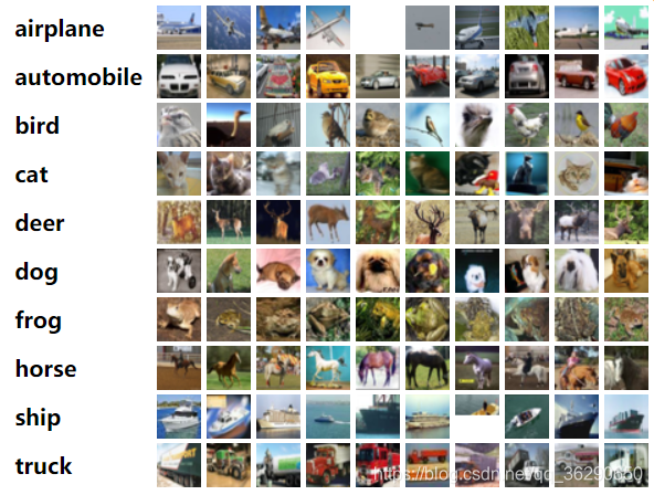
一、CIFAR-10简介

CIFAR-10数据集包含10个类别，共计60000张 32x32 3通道彩色图像。其中每个类别包含6000张图像：训练图像50000张，测试图像10000张。

数据集被分为五个训练批次和一个测试批次。每个测试批次有10000张图像，为每个类别各随机挑出1000张构成；训练批次为随机打乱的剩余图像。某些训练批次可能出现一个类型的图像多于另一个类型的情况，但总体而言，训练批次包含每个类型恰好5000张。

二、说明

图片原格式为32*32 3通道

第一次卷积：卷积核大小为3*3，输出32*32 32通道

第一次池化：最大值池化，输出为16*16 32通道

第二次卷积：卷积核大小为3*3，输出为16*16 64通道

第二次池化：最大值池化，输出为8*8 64通道

全连接层：输入为8*8*64=4096个特征值，隐藏层（一层）包含128条神经元，输出包含10种标签值，经过了one-hot编码

（本项目每一轮会自动保存模型，支持中断后继续训练）

扫描二维码关注公众号，回复： 11949706 查看本文章

三、测试环境

python 版本：3.6

tensorflow版本：1.6.0

系统环境：windows 10 64位  + Visual Studio code

四、资料下载

CIFAR-10官网：http://www.cs.toronto.edu/~kriz/cifar.html

项目代码(附CIFAR-10数据集):  https://pan.baidu.com/s/1T_yC2E60jm9ptjS-CSUPPQ  提取码：0nbg

五、源代码

import urllib.request
import os
import numpy as np
import tarfile
import time
import pickle as pk
import matplotlib.pyplot as plt
import tensorflow as tf
from sklearn.preprocessing import OneHotEncoder

rowData_url = "https://www.cs.toronto.edu/~kriz/cifar-10-python.tar.gz"
filePath_tar = "./data/cifar-10-python.tar.gz"
filePath = "./data/cifar-10-batches-py"

# 检测数据集压缩包是否存在
if not os.path.isfile(filePath_tar):
    print("fail to find row data in disk, we will try to download it from the network...")
    result = urllib.request.urlretrieve(rowData_url, filePath_tar)
    print("downloaded:", result)
else:
    print("success to find the row data from your disk!")

if not os.path.exists("./data/cifar-10-batches-py"):
    tfile = tarfile.open("./data/cifar-10-python.tar.gz")
    tfile.extractall("./data/")
    print("Extracted to \"./data/cifar-10-batches-py\"")
else:
    print("success to find the Directory.")

# def number_to_onehot(num, total_kind=10):
#     result = [0.0 for i in range(total_kind)]
#     if num >= 0 and num < total_kind:
#         result[number] = 1.0

#     return result

def load_CIFAR_batch(fileName):
    # 从磁盘加载并格式化数据
    with open(fileName, "rb") as file:
        data_dict = pk.load(file, encoding="bytes")
        images = data_dict[b"data"]
        labels = data_dict[b"labels"]

        images = images.reshape(10000, 3, 32, 32)                   # 数据转化为(batch,channel,height，width)结构
        images = images.transpose(0, 2, 3, 1)                       # 矩阵转置，调整数据结构为(batch,height,width,channel)
        # labels = [number_to_onehot(i) for i in np.array(labels)]  # 将结果转化为one-hot编码
        labels = np.array(labels)

        return images, labels

def load_CIFAR_data(data_dir):
    "从磁盘加载所有 CIFAR-10 集合数据"

    # 读取训练集
    images_train = []       # 存放训练集输入图像数据
    labels_train = []       # 存放训练集输出标签数据

    for i in range(5):
        file = os.path.join(data_dir, "data_batch_%d" % (i + 1))
        print("loading %s." % file)

        # 通过load_CIFAR_batch()获取批量图像及其对应标签
        image_batch, label_batch = load_CIFAR_batch(file)
        images_train.append(image_batch)
        labels_train.append(label_batch)

        Xtrain = np.concatenate(images_train)  # 两个矩阵拼接成一个矩阵，详见np.concatenate()用法
        Ytrain = np.concatenate(labels_train)

        del image_batch, label_batch  # 及时清理内存

    # 读取测试集数据
    Xtest, Ytest = load_CIFAR_batch(os.path.join(data_dir,"test_batch"))

    return Xtrain, Ytrain, Xtest, Ytest

label_dict = {0: "airplane", 1: "automobile", 2: "bird", 3: "cat", 4: "deer", 5: "dog", 6: "frog", 7: "horse", 8: "ship", 9: "truck"}

# 界面显示预测结果
def plot_images_labels_prediction(images, labels, prediction, start_index, num=15):
    fig = plt.gcf()
    fig.set_size_inches(12, 6)  # 设置显示图片大小

    if num > 15:
        num = 15

    for i in range(0, num):
        ax = plt.subplot(3, 5, i + 1)
        ax.imshow(images[start_index + i], cmap="binary")
        title = str(start_index + i) + ": " + label_dict[np.argmax(labels, axis=1)[start_index + i]]

        if len(prediction) > 0:
            title = title + " => " + label_dict[np.argmax(prediction,axis=1)[start_index + i]]

        # 设置标题
        ax.set_title(title, fontsize=10)

        # 不显示横纵坐标
        ax.set_xticks([])
        ax.set_yticks([])

    #plt.show()


Xtrain, Ytrain, Xtest, Ytest = load_CIFAR_data(data_dir=filePath)
# plt.imshow(Xtrain[6])
# print(Ytrain[0:8])
# plt.show()

# plot_images_labels_prediction(Xtest, Ytest, [], 15)

# 将图像标准化（像素的rgb值转化为0~1之间的float32类型）
Xtrain_normalize = Xtrain.astype("float32") / 255.0
Xtest_normalize = Xtest.astype("float32") / 255.0

# 将标签值进行独热编码
encoder = OneHotEncoder(sparse=False)
encoder.fit([[0], [1], [2], [3], [4], [5], [6], [7], [8], [9]])
# 转化训练集
Ytrain_reshape = Ytrain.reshape(-1, 1)                              # 将Ytrain转化为n行1列的矩阵
Ytrain_onehot = encoder.transform(Ytrain_reshape)
# 转化测试集
Ytest_reshape = Ytest.reshape(-1, 1)  # 将Ytrain转化为n行1列的矩阵
Ytest_onehot = encoder.transform(Ytest_reshape)

# print(Ytrain_onehot.shape)
# print(Ytest_onehot.shape)

# 定义卷积层操作，行列步长均为1，不改变图像大小
def myconv(input,w):
    return tf.nn.conv2d(input, w, strides=[1, 1, 1, 1], padding="SAME")

# 定义池化层操作（最大值池化），步长均为2,故图像规模缩小2*2
def mypool_max(input):
    return tf.nn.max_pool(input,ksize=[1,2,2,1],strides=[1,2,2,1],padding="SAME")

# 定义权值矩阵
def weight(shape):
    # 截断正态分布，标准差为0.1
    return tf.Variable(tf.truncated_normal(shape, stddev=0.1), name="W")

# 定义偏置项
def bias(shape):
    return tf.Variable(tf.constant(0.1,shape=shape),name="b")

with tf.name_scope("input"):
    x=tf.placeholder("float",shape=[None,32,32,3],name="x")

# 卷积层1
with tf.name_scope("conv_1"):
    W1 = weight([3, 3, 3, 32])  # 3*3，输入3通道，输出32通道
    b1 = bias([32])
    conv_1 = myconv(x, W1) + b1     # 卷积运算，加偏置
    conv_1=tf.nn.relu(conv_1)       # 激活函数

# 池化层1
with tf.name_scope("pool_1"):
    pool_1=mypool_max(conv_1)

# 卷积层2
with tf.name_scope("conv_2"):
    W2 = weight([3, 3, 32, 64])
    b2 = bias([64])
    conv_2 = myconv(pool_1, W2) + b2
    conv_2 = tf.nn.relu(conv_2)

# 池化层2
with tf.name_scope("pool_2"):
    pool_2 = mypool_max(conv_2)                 # 此时图片为8*8,64通道

# 全连接层,128条神经元
with tf.name_scope("fc"):
    W3 = weight([4096, 128])                    # 8*8*64个特征值，128条神经元
    b3 = bias([128])
    flat = tf.reshape(pool_2, [-1, 4096])
    h = tf.nn.relu(tf.matmul(flat, W3) + b3)

    h_dropout = tf.nn.dropout(h, keep_prob=0.8) # 减轻或防止过拟合

# 输出层
with tf.name_scope("output"):
    W4 = weight([128, 10])
    b4 = bias([10])

    forward = tf.matmul(h_dropout, W4) + b4
    pred = tf.nn.softmax(forward)


# 定义超参数
learning_rate = 0.0001
train_epochs = 25
max_epochs = 1000
batch_size = 100
total_batch = len(Xtrain) // batch_size
ckpt_dir="./CIFAR10_log/"

epoch_tf = tf.Variable(0, name="epoch", trainable=False)
loss_list_tf = tf.Variable(tf.constant(-1.0, shape=[max_epochs]), dtype=tf.float32, trainable=False)
accuracy_list_tf = tf.Variable(tf.constant(-1.0, shape=[max_epochs]), dtype=tf.float32, trainable=False)
startTime=time.time()

if not os.path.exists(ckpt_dir):
    os.makedirs(ckpt_dir)

# 检测tf.Variable是否足够存储中间损失，精确度
if train_epochs>max_epochs:
    print('"train_epoch" is to big, you can change the "max_epochs", but you will must train your model from the beginning. or you can just smaller your "train_epoch"')
    exit(1)

# 模型定义
with tf.name_scope("optimizer"):
    # 定义标签值占位符
    y = tf.placeholder("float", shape=[None, 10], name="label")

    # 定义损失函数exit
    loss_function = tf.reduce_mean(tf.nn.softmax_cross_entropy_with_logits(logits=forward, labels=y))

    # 定义优化器
    optimizer = tf.train.AdamOptimizer(learning_rate=0.0001).minimize(loss_function)

# 定义准确率
with tf.name_scope("evaluation"):
    correct_prediction = tf.equal(tf.argmax(pred, axis=1), tf.argmax(y, axis=1))
    accuracy = tf.reduce_mean(tf.cast(correct_prediction, tf.float32), reduction_indices=0)

# 获取训练批次数据
def get_train_batch(number, batch_size):
    return Xtrain_normalize[batch_size * number : batch_size * (number + 1)],Ytrain_onehot[batch_size * number : batch_size * (number + 1)]

# 获取训练批次数据
def get_test_batch(number, batch_size):
    return Xtest_normalize[batch_size * number : batch_size * (number + 1)],Ytest_onehot[batch_size * number : batch_size * (number + 1)]


loss_list = [-1.0 for i in range(max_epochs)]
accuracy_list = [-1.0 for i in range(max_epochs)]

saver = tf.train.Saver()
sess = tf.InteractiveSession()

# 训练模型
with tf.name_scope("train_model"):
    sess.run(tf.global_variables_initializer())
    start=0

    ckpt = tf.train.get_checkpoint_state(ckpt_dir)  # 读取上次的训练节点
    if ckpt and ckpt.model_checkpoint_path:
        saver.restore(sess, ckpt.model_checkpoint_path)  # 恢复模型参数
        start = sess.run(epoch_tf)
        loss_list = list(sess.run(loss_list_tf))
        accuracy_list=list(sess.run(accuracy_list_tf))
        print("success to restore the args, training starts from %d epoch" % start)

    if start < train_epochs:        # 判断上次中断是否已经完成模型训练
        for epoch in range(start, train_epochs):
            for i in range(total_batch):
                xs, ys = get_train_batch(epoch, batch_size)
                sess.run(optimizer,feed_dict={x:xs,y:ys})

            loss, acc = sess.run([loss_function, accuracy], feed_dict={x: xs, y: ys})

            # 记录中间损失和精确度
            loss_list[epoch] = loss
            sess.run(tf.assign(loss_list_tf, tf.convert_to_tensor(loss_list)))

            accuracy_list[epoch] = acc
            sess.run(tf.assign(accuracy_list_tf, tf.convert_to_tensor(accuracy_list)))

            sess.run(tf.assign(epoch_tf,epoch+1))
            saver.save(sess, os.path.join(ckpt_dir, "CIFAR10_model_{:06d}.ckpt").format(epoch+1))


            print("epoch %d: "%(epoch+1),"loss=",loss," accuracy=",acc)

    print("Train finished takes %.2fs"%(time.time()-startTime))

# 绘制损失、精确度变化曲线

def get_real_list(input):
    output=[]
    for i in input:
        if i > 0:
            output.append(i)
        else:
            break
    return output

with tf.name_scope("plot_loss_acc"):
    plt.rcParams['font.sans-serif'] = ['FangSong']  # 指定默认字体
    plt.rcParams['axes.unicode_minus'] = False  # 解决保存图像时'-'显示为方块的问题

    plt.figure(1)
    loss_img = plt.subplot(1, 2, 1)
    plt.plot(get_real_list(loss_list))
    loss_img.set_title("损失变化曲线")

    accuracy_img = plt.subplot(1, 2, 2)
    plt.plot(get_real_list(accuracy_list))
    accuracy_img.set_title("精确度变化曲线")

    #plt.show()

test_batch_size=1000
with tf.name_scope("test_model"):
    loss_test = 0.0
    accuracy_test = 0.0
    for i in range(len(Xtest) // test_batch_size):
        xs,ys=get_test_batch(i,batch_size)
        loss, acc = sess.run([loss_function, accuracy], feed_dict={x: xs, y: ys})

        loss_test += loss
        accuracy_test += acc

    loss_test /= len(Xtest) / test_batch_size
    accuracy_test /= len(Xtest) / test_batch_size

    print("final result: loss=%d, accuracy=%.02f" % (loss_test, accuracy_test))


# 抽取样本图显示
with tf.name_scope("plot_real_image_test"):
    startIndex = 0

    epoch = startIndex // 15
    start = startIndex % 15
    xs, ys = get_test_batch(epoch, 15)
    prediction = sess.run(pred, feed_dict={x: xs, y: ys})

    plt.figure(2)
    plot_images_labels_prediction(Xtest[startIndex: startIndex + 15], Ytest_onehot[startIndex: startIndex + 15], prediction, start)

    plt.show()